什么是CP和CPK
- 格式:doc
- 大小:5.18 MB
- 文档页数:17

CP和CPK介紹CP(或Cpk)是英文Process Capability index縮寫,漢語譯作工序能力指數,也有譯作工藝能力指數過程能力指數。
工序能力指數,是指工序在一定時間裏,處於控制狀態(穩定狀態)下的實際加工能力。
它是工序固有的能力,或者說它是工序保證品質的能力。
這裡所指的工序,是指操作者、機器、原材料、工藝方法和生產環境等五個基本品質因素綜合作用的過程,也就是產品品質的生產過程。
產品品質就是工序中的各個品質因素所起作用的綜合表現。
對於任何生產過程,產品品質總是分散地存在著。
若工序能力越高,則產品品質特性值的分散就會越小;若工序能力越低,則產品品質特性值的分散就會越大。
那麼,應當用一個什麼樣的量,來描述生產過程所造成的總分散呢?通常,都用6σ(即μ+3σ)來表示工序能力:工序能力=6σ若用符號P來表示工序能力,則:P=6σ式中:σ是處於穩定狀態下的工序的標準偏差工序能力是表示生產過程客觀存在著分散的一個參數。
但是這個參數能否滿足產品的技術要求,僅從它本身還難以看出。
因此,還需要另一個參數來反映工序能力滿足產品技術要求(公差、規格等品質標準)的程度。
這個參數就叫做工序能力指數。
它是技術要求和工序能力的比值,即工序能力指數=技術要求/工序能力當分佈中心與公差中心重合時,工序能力指數記為Cp。
當分佈中心與公差中心有偏離時,工序能力指數記為Cpk。
運用工序能力指數,可以幫助我們掌握生產過程的品質水準。
工序能力指數的判斷工序的品質水準按Cp值可劃分為五個等級。
按其等級的高低,在管理上可以作出相應的判斷和處置(見表1)。
該表中的分級、判斷和處置對於Cpk也同樣適用。
表1 工序能力指數的分級判斷和處置參考表。
什么是CP和CPKCP(或Cpk)是英文Process Capability index缩写,汉语译作工序能力指数,也有译作工艺能力指数, 过程能力指数。
工序能力指数,是指工序在一定时间里,处于控制状态(稳定状态)下的实际加工能力。
它是工序固有的能力,或者说它是工序保证质量的能力。
这里所指的工序,是指操作者、机器、原材料、工艺方法和生产环境等五个基本质量因素综合作用的过程,也就是产品质量的生产过程。
产品质量就是工序中的各个质量因素所起作用的综合表现。
对于任何生产过程,产品质量总是分散地存在着。
若工序能力越高,则产品质量特性值的分散就会越小;若工序能力越低,则产品质量特性值的分散就会越大。
那么,应当用一个什么样的量,来描述生产过程所造成的总分散呢?通常,都用6σ(即μ+3σ)来表示工序能力:工序能力=6σ若用符号P来表示工序能力,则:P=6σ式中:σ是处于稳定状态下的工序的标准偏差工序能力是表示生产过程客观存在着分散的一个参数。
但是这个参数能否满足产品的技术要求,仅从它本身还难以看出。
因此,还需要另一个参数来反映工序能力满足产品技术要求(公差、规格等质量标准)的程度。
这个参数就叫做工序能力指数。
它是技术要求和工序能力的比值,即工序能力指数=技术要求/工序能力当分布中心与公差中心重合时,工序能力指数记为Cp。
当分布中心与公差中心有偏离时,工序能力指数记为Cpk。
运用工序能力指数,可以帮助我们掌握生产过程的质量水平。
工序能力指数的判断工序的质量水平按Cp值可划分为五个等级。
按其等级的高低,在管理上可以作出相应的判断和处置(见表1)。
该表中的分级、判断和处置对于Cpk也同样适用。
表1工序能力指数的分级判断和处置参考表Ppk, Cpk, Cmk 三者的区别及计算1、首先我们先说明Pp、Cp两者的定义及公式Cp(Capability Indies of Process):稳定过程的能力指数,定义为容差宽度除以过程能力,不考虑过程有无偏移,一般表达式为:Pp(Performance Indies of Process):过程性能指数,定义为不考虑过程有无偏移时,容差范围除以过程性能,一般表达式为:(该指数仅用来与Cp及Cpk对比,或/和Cp、Cpk一起去度量和确认一段时间内改进的优先次序)CPU:稳定过程的上限能力指数,定义为容差范围上限除以实际过程分布宽度上限,CPL:稳定过程的下限能力指数,定义为容差范围下限除以实际过程分布宽度下限,2、现在我们来阐述Cpk、Ppk的含义Cpk:这是考虑到过程中心的能力(修正)指数,定义为CPU与CPL的最小值。
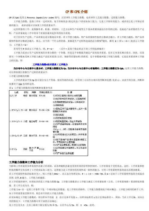
过程能力和过程能力指数(CP 和CPK)相关知识一、什么是过程能力和过程能力指数(英文Process Capability Index)1、过程能力(或工序能力)C P,是指过程的加工质量满足技术标准的能力,它是衡量过程加工内在一致性的。
过程能力决定于质量因素,即人、机、料、法、环、测,而与规范无关。
2、C P值的大小即可定量计算出该工序的不合格品率,所以工序能力C P的大小可以反映过程加工质量满足产品技术要求的程度,也即企业产品的控制范围满足客户要求的程度。
3、C PK:Process Capability Index(K是偏移量),称为过程能力指数(指过程的固有过程能力指数),表示过程能力满足技术标准的程度。
二、Cp、Cpk的计算方法在品质特性值属于计量值数据的情况下,工序能力指数的计算方法如下:1、当给定双向公差,品质数据分布中心( X ) 与公差中心( M ) 相一致时,用符号C P 表示。
C P(工序能力指数)=T(质量特性规格界限)/6σ(工序能力)T=T U–T LT U为公差上限,T L为公差下限;2、当给定双向公差,品质数据分布中心( X ) 与公差中心( M ) 不一致时,即存在中心偏移量(ε)时,用符号C PK表示。
C PK =(1–k)C Pk= 2ε/Tε=|M–X|C PK =(T–2ε)/6σσ是通过计算标准偏差的方法计算(可由电脑自动生成,在统计函数SDTEV A中)3、举例说明以选取新郑分厂7月2日313晨班生产101100412500(牛面115g香辣)品种时所抽取的119120119117116117118117117118 117116117117119118119121120119 119117119117117119117118118118 119118117117118119118117119118 118117117117117118118120119118 117116117117118117120118118118 117117117121120118118118118117标准偏差σ1.1233平均值X118.08标准值M116.5最大值T U120.5最小值T L112.5T=T U–T L=120.5–112.5=8ε=|M–X|=|116.5–118.08|=1.58σ=1.1233 k=2ε / T=0.395C P =T/6σ=8/6*1.1233=1.187C PK=(T–2ε)/6σ=(8–2*1.58)/6*1.1233 = 0.718当过程中心值偏移时三、过程能力指数C P的评价参考C P≥1.67 属Ⅰ级,过程能力过高(视具体情况而定)。
cp和cpk的标准CP和CPK的标准。
在品质管理领域中,CP和CPK是两个重要的统计指标,用于评估过程的稳定性和能力。
它们可以帮助我们了解生产过程的偏差程度,以及产品是否符合客户的要求。
本文将对CP和CPK的定义、计算方法以及应用进行详细介绍。
CP是过程能力指数,用于衡量过程的稳定性。
它是通过比较过程的偏差范围和规格范围来评估过程的能力。
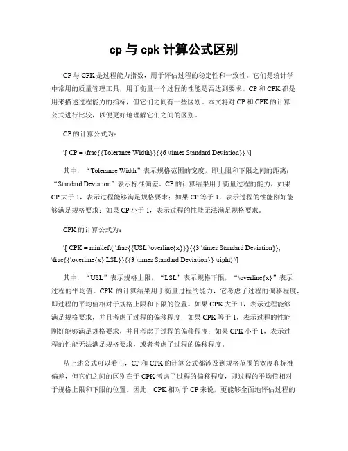
CP的计算公式为:\[ CP = \frac{USL LSL}{6\sigma} \]其中,USL为规格上限,LSL为规格下限,σ为过程标准差。
CP的数值越大,表示过程的稳定性越高,产品的质量波动越小。
CPK是过程潜在能力指数,它不仅考虑了过程的稳定性,还考虑了过程的中心位置。
CPK的计算公式为:\[ CPK = min\left(\frac{USL \mu}{3\sigma}, \frac{\mu LSL}{3\sigma}\right) \]其中,μ为过程的均值。
CPK的数值越大,表示过程的能力越强,产品的质量波动越小。
CP和CPK的应用可以帮助我们进行过程改进和质量控制。
当CP和CPK的数值低于1.33时,说明过程的能力不足,需要采取措施进行改进。
通过对过程参数的调整和控制,可以提高CP和CPK的数值,从而提高产品的质量稳定性和一致性。
除了衡量过程的稳定性和能力,CP和CPK还可以用于制定产品规格和质量标准。
通过分析CP和CPK的数值,可以确定产品的合格范围,为生产过程和质量控制提供依据。
总之,CP和CPK是衡量过程稳定性和能力的重要指标,它们对于提高产品质量、降低成本、提高客户满意度具有重要意义。
通过合理计算和应用CP和CPK,可以帮助企业实现持续改进和持续稳定的生产过程,从而获得竞争优势。
什么是CP和CPKCP(或Cpk)是英文Process Capability index缩写,汉语译作工序能力指数,也有译作工艺能力指数, 过程能力指数。
工序能力指数,是指工序在一定时间里,处于控制状态(稳定状态)下的实际加工能力。
它是工序固有的能力,或者说它是工序保证质量的能力。
这里所指的工序,是指操作者、机器、原材料、工艺方法和生产环境等五个基本质量因素综合作用的过程,也就是产品质量的生产过程。
产品质量就是工序中的各个质量因素所起作用的综合表现。
对于任何生产过程,产品质量总是分散地存在着。
若工序能力越高,则产品质量特性值的分散就会越小;若工序能力越低,则产品质量特性值的分散就会越大。
那么,应当用一个什么样的量,来描述生产过程所造成的总分散呢?通常,都用6σ(即μ+3σ)来表示工序能力:工序能力=6σ若用符号P来表示工序能力,则:P=6σ式中:σ是处于稳定状态下的工序的标准偏差工序能力是表示生产过程客观存在着分散的一个参数。
但是这个参数能否满足产品的技术要求,仅从它本身还难以看出。
因此,还需要另一个参数来反映工序能力满足产品技术要求(公差、规格等质量标准)的程度。
这个参数就叫做工序能力指数。
它是技术要求和工序能力的比值,即工序能力指数=技术要求/工序能力当分布中心与公差中心重合时,工序能力指数记为Cp。
当分布中心与公差中心有偏离时,工序能力指数记为Cpk。
运用工序能力指数,可以帮助我们掌握生产过程的质量水平。
工序能力指数的判断工序的质量水平按Cp值可划分为五个等级。
按其等级的高低,在管理上可以作出相应的判断和处置(见表1)。
该表中的分级、判断和处置对于Cpk也同样适用。
表1工序能力指数的分级判断和处置参考表Ppk, Cpk, Cmk 三者的区别及计算1、首先我们先说明Pp、Cp两者的定义及公式Cp(Capability Indies of Process):稳定过程的能力指数,定义为容差宽度除以过程能力,不考虑过程有无偏移,一般表达式为:Pp(Performance Indies of Process):过程性能指数,定义为不考虑过程有无偏移时,容差范围除以过程性能,一般表达式为:(该指数仅用来与Cp及Cpk对比,或/和Cp、Cpk一起去度量和确认一段时间内改进的优先次序)CPU:稳定过程的上限能力指数,定义为容差范围上限除以实际过程分布宽度上限,CPL:稳定过程的下限能力指数,定义为容差范围下限除以实际过程分布宽度下限,2、现在我们来阐述Cpk、Ppk的含义Cpk:这是考虑到过程中心的能力(修正)指数,定义为CPU与CPL的最小值。
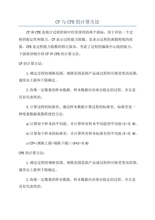
CP与CPK的计算方法CP和CPK是统计过程控制中经常使用的两个指标,用于评估一个过程的稳定性和能力。
CP表示过程能力指数,是表示过程的离散程度的度量。
CPK是过程能力指数的修正版本,考虑了过程的偏离中心线的能力。
下面将详细介绍CP和CPK的计算方法。
CP的计算方法:1.确定过程的规格范围。
规格范围是指产品或过程的可接受变动范围,通常由上限和下限确定。
2.收集一定数量的样本数据。
样本数据应该来自稳定的过程,并且是具有代表性的。
3.计算过程的标准差。
通过样本数据计算过程的标准差。
标准差是一种度量数据离散程度的方法。
a)计算每个样本的平均值,并计算所有样本平均值的平均值(X-双M)。
b)计算每个样本的标准差,并计算所有样本标准差的平均值(S-双M)。
c)CP=(规格上限-规格下限)/(6*S-双M)CPK的计算方法:1.确定过程的规格范围。
规格范围是指产品或过程的可接受变动范围,通常由上限和下限确定。
2.收集一定数量的样本数据。
样本数据应该来自稳定的过程,并且是具有代表性的。
3.计算过程的标准差和平均值。
通过样本数据计算过程的标准差和平均值。
4.计算规格上限、规格下限与过程平均值之间的距离。
a)USL-过程平均值=d1b)过程平均值-LSL=d25.根据标准差的两倍计算过程的变异范围。
a)2*标准差=d36.根据d1、d2和d3计算CPK。
a) CPK = min(d1 / 3*d3, d2 / 3*d3)CP和CPK的解读:CP和CPK都是表示过程能力的指标,它们的值越大,说明过程的稳定性和能力越好。
1.如果CPK>1,表示过程的能力很好,能够满足规格要求。
2.如果CPK<1,表示过程的能力不足,需要改进过程以满足规格要求。
3.如果CPK<0.67,表示过程严重不稳定,需要进行根本性的改进。
总结:CP和CPK是用于评估一个过程的稳定性和能力的指标,通过CP和CPK的计算,可以了解到过程的离散程度和一致性。
CP和CPK介绍CP(或Cpk)是英文Process Capability index缩写,汉语译作工序能力指数,也有译作工艺能力指数、过程能力指数。
工序能力指数,是指工序在一定时间里,处于控制状态(稳定状态)下的实际加工能力。
它是工序固有的能力,或者说它是工序保证质量的能力。
或者说他可以体现工序的质量水平。
这里所指的工序,是指操作者、机器、原材料、工艺方法和生产环境等五个基本质量因素综合作用的过程,也就是产品质量的生产过程。
产品质量就是工序中的各个质量因素所起作用的综合表现。
对于任何生产过程,产品质量总是分散地存在着。
若工序能力越高,则产品质量特性值的分散就会越小;若工序能力越低,则产品质量特性值的分散就会越大。
那么,应当用一个什么样的量,来描述生产过程所造成的总分散呢?通常,都用6σ(即μ+3σ)来表示工序能力:工序能力=6σ若用符号P来表示工序能力,则:P=6σ(式中σ是处于稳定状态下的工序的标准偏差)工序能力是表示生产过程客观存在着分散的一个参数。
但是这个参数能否满足产品的技术要求,仅从它本身还难以看出。
因此,还需要另一个参数来反映工序能力满足产品技术要求(公差、规格等质量标准)的程度。
这个参数就叫做工序能力指数。
它是技术要求和工序能力的比值,即工序能力指数=技术要求/工序能力当分布中心与公差中心重合时,工序能力指数记为Cp。
当分布中心与公差中心有偏离时,工序能力指数记为Cpk。
运用工序能力指数,可以帮助我们掌握生产过程的质量水平。
工序能力指数的判断工序的质量水平按Cp值可划分为五个等级。
按其等级的高低,在管理上可以作出相应的判断和处置(见表1)。
该表中的分级、判断和处置对于Cpk也同样适用。
表1 工序能力指数的分级判断和处置参考表工序能力指数和工序能力分析当影响工序质量的各种系统性因素已经消除,而各种随机因素也受到有效的管理和控制时,工序质量处于受控状态。
这时,工序质量和特性值的概率分布反映了工序的实际加工能力。
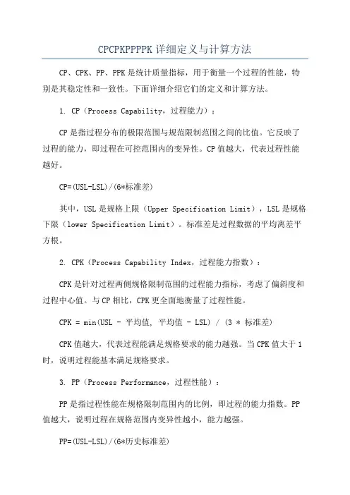
CPCPKPPPPK详细定义与计算方法CP、CPK、PP、PPK是统计质量指标,用于衡量一个过程的性能,特别是其稳定性和一致性。
下面详细介绍它们的定义和计算方法。
1. CP(Process Capability,过程能力):CP是指过程分布的极限范围与规范限制范围之间的比值。
它反映了过程的能力,即过程在可控范围内的变异性。
CP值越大,代表过程性能越好。
CP=(USL-LSL)/(6*标准差)其中,USL是规格上限(Upper Specification Limit),LSL是规格下限(lower Specification Limit)。
标准差是过程数据的平均离差平方根。
2. CPK(Process Capability Index,过程能力指数):CPK是针对过程两侧规格限制范围的过程能力指标,考虑了偏斜度和过程中心值。
与CP相比,CPK更全面地衡量了过程性能。
CPK = min(USL - 平均值, 平均值 - LSL) / (3 * 标准差)CPK值越大,代表过程能满足规格要求的能力越强。
当CPK值大于1时,说明过程能基本满足规格要求。
3. PP(Process Performance,过程性能):PP是指过程性能在规格限制范围内的比例,即过程的能力指数。
PP 值越大,说明过程在规格范围内变异性越小,能力越强。
PP=(USL-LSL)/(6*历史标准差)其中,历史标准差是过去的过程数据的平均离差平方根。
4. PPK(Process Performance Index,过程性能指数):PPK是过程指标,类似于PP,但它也考虑了过程中心值。
PPK比PP更全面地评估了过程的性能。
PPK = min(USL - 平均值, 平均值 - LSL) / (3 * 历史标准差)PPK值越大,代表过程能满足规格要求的概率越高。
当PPK值大于1时,表明过程性能能够基本满足规格要求。
计算方法中常涉及的术语解释:-规格上限(USL):产品或过程的上限要求。

cp与cpk计算公式区别CP与CPK是过程能力指数,用于评估过程的稳定性和一致性。
它们是统计学中常用的质量管理工具,用于衡量一个过程的性能是否达到要求。
CP和CPK都是用来描述过程能力的指标,但它们之间有一些区别。
本文将对CP和CPK的计算公式进行比较,以便更好地理解它们之间的区别。
CP的计算公式为:\[ CP = \frac{{Tolerance Width}}{{6 \times Standard Deviation}} \]其中,“Tolerance Width”表示规格范围的宽度,即上限和下限之间的距离;“Standard Deviation”表示标准偏差。
CP的计算结果用于衡量过程的能力,如果CP大于1,表示过程能够满足规格要求;如果CP等于1,表示过程的性能刚好能够满足规格要求;如果CP小于1,表示过程的性能无法满足规格要求。
CPK的计算公式为:\[ CPK = min\left( \frac{{USL \overline{x}}}{{3 \times Standard Deviation}},\frac{{\overline{x} LSL}}{{3 \times Standard Deviation}} \right) \]其中,“USL”表示规格上限,“LSL”表示规格下限,“\overline{x}”表示过程的平均值。
CPK的计算结果用于衡量过程的能力,它考虑了过程的偏移程度,即过程的平均值相对于规格上限和下限的位置。
如果CPK大于1,表示过程能够满足规格要求,并且考虑了过程的偏移程度;如果CPK等于1,表示过程的性能刚好能够满足规格要求,并且考虑了过程的偏移程度;如果CPK小于1,表示过程的性能无法满足规格要求,或者考虑了过程的偏移程度。
从上述公式可以看出,CP和CPK的计算公式都涉及到规格范围的宽度和标准偏差,但它们之间的区别在于CPK考虑了过程的偏移程度,即过程的平均值相对于规格上限和下限的位置。
cp -r命令的用法
cp和cpk的区别:cp表示产品过程的精密程度,不考虑中心值的位置;cpk表示产品满足规格的能力,考虑中心值的位置。
通常情况下,cp和cpk一起使用。
什么是cp、cpk
cp就是指过程满足用户技术建议的能力,常用客户令人满意的偏差范围除以六倍的西格玛的结果去则表示。
t=允许最大值(tu)-允许最小值(tl)
cp=t/(6*σ)
所以σ越小,其cp值越大,则过程技术能力越好。
cpk就是指过程平均值与产品标准规格出现偏转(ε)的大小,常用客户令人满意的下限偏差值乘以平均值和平均值乘以上限偏差值中数值大的一个,再除以三倍的西格玛的结果去则表示。
cpk=min(tu-μ,μ-tl)/(3*σ)
或者cpk=(1-k)*cp,其中k=ε/(t/2)
通常状况下,质量特性值分布的总体标准差(σ)是未知的,所以应采用样本标准差(s)来代替。
cp与cpk的标准CP与CPK的标准。
在制造业中,CP和CPK是两个重要的质量管理指标,它们用来评估一个过程的稳定性和能力。
CP和CPK的计算可以帮助企业了解产品质量的稳定性和一致性,从而及时进行调整和改进。
本文将重点介绍CP和CPK的定义、计算方法以及如何应用这两个指标来提高生产质量。
CP和CPK的定义。
CP是过程能力指数,用来评估过程的稳定性。
它是通过测量过程的分布宽度和规格限的关系来确定的。
CP的计算公式为,CP = (USL-LSL)/(6标准差),其中USL为规格上限,LSL为规格下限,标准差是过程的标准差。
CP的数值越大,说明过程的稳定性越好。
CPK是过程能力指数的修正值,它同时考虑了过程的中心位置和分布的偏移。
CPK的计算公式为,CPK = min[(USL-μ)/(3标准差),(μ-LSL)/(3标准差)],其中μ为过程的平均值。
CPK的数值越大,说明过程的能力越强,能够更好地满足规格要求。
CP和CPK的计算方法。
要计算CP和CPK,首先需要收集过程数据,包括规格上限和下限,以及过程的标准差和平均值。
然后根据上面的公式进行计算,得到CP和CPK的数值。
通过这些数值,可以判断过程的稳定性和能力,从而采取相应的措施进行改进。
如何应用CP和CPK来提高生产质量。
通过计算CP和CPK,企业可以了解产品质量的稳定性和一致性,从而及时发现和解决生产过程中的问题。
如果CP和CPK的数值较低,说明过程存在较大的变异性,需要进一步分析原因并采取改进措施,以提高过程的稳定性和能力。
另外,CP和CPK的计算结果也可以帮助企业确定产品的合格率,从而更好地控制产品质量。
总结。
CP和CPK是评估过程稳定性和能力的重要指标,它们可以帮助企业了解产品质量的情况,并及时进行调整和改进。
通过计算CP和CPK,企业可以更好地管理生产过程,提高产品质量,满足客户需求。
因此,企业应该重视CP和CPK的应用,不断优化生产过程,提高竞争力。
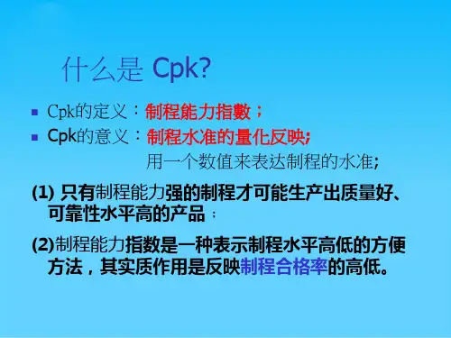
但是关于过程能力指数,还是有很多令初学者不解的疑问,甚至略感神秘。
今天就Cp与Cpk的10个疑问给大家分析一下,帮助大家揭开其神秘面纱。
1. Cp与Cpk都被称为过程能力指数,二者的区别是什么呢?首先要介绍两个术语“无偏”和“有偏”。
当数据的分布中心与公差中心重合,称为无偏。
而无偏情形下的过程能力指数就是Cp,也称理论上的过程能力指数;当数据的分布中心与公差中心不重合,称为有偏。
而有偏情形下的过程能力指数就是Cpk,也称实际上的过程能力指数。
在实际的工作当中,我们研究的是有偏过程能力指数Cpk,以此作为衡量过程能力的指标。
2. 为什么Cp有另一个名字叫“精密度”?大家知道,Cp=T/6σ(T为规格的公差范围,σ为标准差)。
从数学角度上来讲,Cp的大小与T和σ有关。
但从质量管理角度来看,Cp只与σ有关,为什么这么说呢?因为产品规格的公差范围T是人为设定的(通常由设计工程师制定),而如何提高过程能力指数Cp,就要从如何减小σ、提高产品加工精度方面下功夫,以满足设计的公差要求,而不能直接找设计部门要求放宽公差带。
正因为Cp 只与标准差σ有关,所以Cp的另一个名字,叫“精密度”。
3. Cp计算公式的内涵是什么?上面提到了无偏过程能力指数Cp=T/6σ,这个公式代表了什么意思呢?要揭晓答案,就要提到SPC的核心工具——控制图,因为控制图通常都是与Cp、Cpk分不开的。
在计量控制图中,根据3σ最经济的原则,控制上限UCL与控制下限LCL 之间的宽度为6倍σ。
控制限与规格限的关系如下所示:既然控制限在规格限的范围之内,我们再来看下面这张图:上图中,T为规格限的宽度,即公差范围;6σ为控制限的宽度。
所以,无偏过程能力指数Cp就是产品设计的规格限宽度与加工过程控制限宽度的比值,即Cp=T/6σ。
规格限的宽度是一定的,所以加工能力的大小取决于控制限的宽度,宽度越窄,加工的精度就越高,Cp的数值就越大。
4. Cpk与Cp只有一“k”之差,那么k又是什么呢?k的起源可以追溯到20世纪70年代的日本。
CPCPK计算原理详解CP和CPK是统计过程控制(SPC)中用来评估过程的能力和稳定性的两个指标。
CP指标表示了过程的能力,即过程可以生产符合规格要求的产品的潜力。
CPK指标则表示了过程的稳定性,即过程在长期运行中能够保持生产符合规格要求的产品的能力。
CP和CPK的计算原理基于统计学中的过程能力指数(Process Capability Index)。
过程能力指数是根据过程的离散度和规格宽度来评估过程的能力。
它可以帮助我们判断过程是否足够稳定,以生产出符合规格要求的产品。
CP的计算公式为:CP=(上限规格值-下限规格值)/(6*标准差)其中,上限规格值和下限规格值分别表示产品规格的上下限值,标准差表示过程的离散度。
CP的数值越大,表示过程的能力越好;反之,数值越小,表示过程的能力越差。
CPK的计算公式为:CPK = min((上限规格值 - 过程平均值) / (3 * 标准差), (过程平均值 - 下限规格值) / (3 * 标准差))CPK是基于过程的平均值、上下限规格值和标准差来计算的。
CPK的数值越大,表示过程的稳定性越好;反之,数值越小,表示过程的稳定性越差。
当CP和CPK的数值大于1时,表示过程的能力和稳定性都比较好,可以生产符合规格要求的产品。
当CP和CPK的数值小于1时,表示过程的能力和稳定性不够,需要对过程进行改进。
CP和CPK的计算原理可以帮助我们了解过程的能力和稳定性,从而指导我们进行质量控制和过程改进。
通过定期计算CP和CPK指标,并与规格要求进行对比,可以帮助我们发现过程中的问题并采取相应的措施,以提高过程的能力和稳定性。
需要注意的是,CP和CPK只是过程能力的评估指标,不能替代质量控制和过程改进的具体方法和措施。
因此,在实际应用中,还需要结合其他统计分析方法和质量管理工具,全面评估和改进过程的能力和稳定性。
过程能力和过程能力指数(CP 和CPK)相关知识一、什么是过程能力和过程能力指数(英文Process Capability Index)1、过程能力(或工序能力)CP,是指过程的加工质量满足技术标准的能力,它是衡量过程加工内在一致性的。
过程能力决定于质量因素,即人、机、料、法、环、测,而与规范无关。
2、CP 值的大小即可定量计算出该工序的不合格品率,所以工序能力CP的大小可以反映过程加工质量满足产品技术要求的程度,也即企业产品的控制范围满足客户要求的程度。
3、CPK:Process Capability Index(K是偏移量),称为过程能力指数(指过程的固有过程能力指数),表示过程能力满足技术标准的程度。
二、Cp、Cpk的计算方法在品质特性值属于计量值数据的情况下,工序能力指数的计算方法如下:1、当给定双向公差,品质数据分布中心 ( X ) 与公差中心 ( M ) 相一致时,用符号CP 表示。
CP(工序能力指数)=T(质量特性规格界限)/6σ(工序能力)T=TU –TLT U 为公差上限,TL为公差下限;2、当给定双向公差,品质数据分布中心 ( X ) 与公差中心 ( M ) 不一致时,即存在中心偏移量 (ε)时,用符号 CPK表示。
C PK =(1–k)CPk= 2ε/Tε=|M–X|CPK=(T–2ε)/6σσ是通过计算标准偏差的方法计算(可由电脑自动生成,在统计函数SDTEVA中)3、举例说明以选取新郑分厂7月2日313晨班生产(牛面115g香辣)品种时所抽取的样本数据为例:118117120117119118118117119118 117120119118117117117120119118 119117118119118117121120118117 119120117117118117118118117117 118119120117117118117117117118 119120119117116117118117117118 117116117117119118119121120119 119117119117117119117118118118 119118117117118119118117119118 118117117117117118118120119118 117116117117118117120118118118 117117117121120118118118118117标准偏差σ平均值X标准值M最大值T U最小值T LT=TU –TL=–=8ε=|M–X|=|–|=σ=k=2ε / T=CP=T/6σ=8/6*=CPK=(T–2ε)/6σ=(8–2*)/6* = 当过程中心值偏移时三、过程能力指数C P的评价参考从上述新郑的事例可以看出新郑分厂7月2日313晨班生产(牛面115g香辣)的CP值为,在>CP ≥的范围之内,整体样本的中心向TU方向偏移,应加以适当的调整和控制。
C P K计算公式-CAL-FENGHAI.-(YICAI)-Company One1什么是CP和CPK(工序能力指数) CP(或CPK)是英文Process Capability index缩写,汉语译作工序能力指数,也有译作工艺能力指数过程能力指数。
工序能力指数,是指工序在一定时间里,处于控制状态(稳定状态)下的实际加工能力。
它是工序固有的能力,或者说它是工序保证质量的能力。
对于任何生产过程,产品质量总是分散地存在着。
若工序能力越高,则产品质量特性值的分散就会越小;若工序能力越低,则产品质量特性值的分散就会越大。
那么,应当用一个什么样的量,来描述生产过程所造成的总分散呢通常,都用6σ(即μ+3σ)来表示工序能力:工序能力=6σ若用符号P 来表示工序能力,则:P=6σ式中:σ是处于稳定状态下的工序的标准偏差工序能力是表示生产过程客观存在着分散的一个参数。
但是这个参数能否满足产品的技术要求,仅从它本身还难以看出。
因此,还需要另一个参数来反映工序能力满足产品技术要求(公差、规格等质量标准)的程度。
这个参数就叫做工序能力指数。
它是技术要求和工序能力的比值,即工序能力指数=技术要求/工序能力当分布中心与公差中心重合时,工序能力指数记为Cp。
当分布中心与公差中心有偏离时,工序能力指数记为CPK。
运用工序能力指数,可以帮助我们掌握生产过程的质量水平。
工序能力指数的判断工序的质量水平按Cp值可划分为五个等级。
按其等级的高低,在管理上可以作出相应的判断和处置(见表1)。
该表中的分级、判断和处置对于CPK也同样适用。
表1 工序能力指数的分级判断和处置参考表 Cp值级别判断双侧公差范(T) 处置 Cp> 特级能力过高 T>106 (1)可将公差缩小到约土46的范围 (2)允许较大的外来波动,以提高效率 (3)改用精度差些的设备,以降低成本 (4)简略检验≥一级能力充分 T=86—106 (1)若加工件不是关键零件,允许一定程度的外来波动(2)简化检验 (3)用控制图进行控制≥Cp> 二级能力尚可 T=66—86 (1)用控制图控制,防止外来波动 (2)对产品抽样检验,注意抽样方式和间隔 (3)Cp—1.0时,应检查设备等方面的情示器≥Cp> 三级能力不足 T=46—66 (1)分析极差R过大的原因,并采取措施(2)若不影响产品最终质量和装配工作,可考虑放大公差范围 (3)对产品全数检查,或进行分级筛选 >Cp 1、首先我们先说明Pp、Cp两者的定义及公式 Cp(Capability Indies of Process):稳定过程的能力指数,定义为容差宽度除以过程能力,不考虑过程有无偏移,一般表达式为: Cpk, Ca, Cp三者的关系: Cpk = Cp *( 1 -┃Ca┃),Cpk 是Ca及Cp两者的中和反应,Ca反应的是位置关系(集中趋势),Cp反应的是散布关系(离散趋势) 4。
什么是CP和CPKCP(或Cpk)是英文Process Capability index缩写,汉语译作工序能力指数,也有译作工艺能力指数, 过程能力指数。
工序能力指数,是指工序在一定时间里,处于控制状态(稳定状态)下的实际加工能力。
它是工序固有的能力,或者说它是工序保证质量的能力。
这里所指的工序,是指操作者、机器、原材料、工艺方法和生产环境等五个基本质量因素综合作用的过程,也就是产品质量的生产过程。
产品质量就是工序中的各个质量因素所起作用的综合表现。
对于任何生产过程,产品质量总是分散地存在着。
若工序能力越高,则产品质量特性值的分散就会越小;若工序能力越低,则产品质量特性值的分散就会越大。
那么,应当用一个什么样的量,来描述生产过程所造成的总分散呢?通常,都用6σ(即μ+3σ)来表示工序能力:工序能力=6σ若用符号P来表示工序能力,则:P=6σ式中:σ是处于稳定状态下的工序的标准偏差工序能力是表示生产过程客观存在着分散的一个参数。
但是这个参数能否满足产品的技术要求,仅从它本身还难以看出。
因此,还需要另一个参数来反映工序能力满足产品技术要求(公差、规格等质量标准)的程度。
这个参数就叫做工序能力指数。
它是技术要求和工序能力的比值,即工序能力指数=技术要求/工序能力当分布中心与公差中心重合时,工序能力指数记为Cp。
当分布中心与公差中心有偏离时,工序能力指数记为Cpk。
运用工序能力指数,可以帮助我们掌握生产过程的质量水平。
工序能力指数的判断工序的质量水平按Cp值可划分为五个等级。
按其等级的高低,在管理上可以作出相应的判断和处置(见表1)。
该表中的分级、判断和处置对于Cpk也同样适用。
表1工序能力指数的分级判断和处置参考表Ppk, Cpk, Cmk 三者的区别及计算1、首先我们先说明Pp、Cp两者的定义及公式Cp(Capability Indies of Process):稳定过程的能力指数,定义为容差宽度除以过程能力,不考虑过程有无偏移,一般表达式为:Pp(Performance Indies of Process):过程性能指数,定义为不考虑过程有无偏移时,容差范围除以过程性能,一般表达式为:(该指数仅用来与Cp及Cpk对比,或/和Cp、Cpk一起去度量和确认一段时间内改进的优先次序)CPU:稳定过程的上限能力指数,定义为容差范围上限除以实际过程分布宽度上限,CPL:稳定过程的下限能力指数,定义为容差范围下限除以实际过程分布宽度下限,2、现在我们来阐述Cpk、Ppk的含义Cpk:这是考虑到过程中心的能力(修正)指数,定义为CPU与CPL的最小值。
它等于过程均值与最近的规范界限之间的差除以过程总分布宽度的一半。
Ppk:这是考虑到过程中心的性能(修正)指数,定义为:或的最小值。
其实,公式中的K是定义分布中心μ与公差中心M的偏离度,μ与M的偏离为ε=| M-μ| ,3、公式中标准差的不同含义①在Cp、Cpk中,计算的是稳定过程的能力,稳定过程中过程变差仅由普通原因引起,公式中的标准差可以通过控制图中的样本平均极差估计得出:因此,Cp、Cpk一般与控制图一起使用,首先利用控制图判断过程是否受控,如果过程不受控,要采取措施改善过程,使过程处于受控状态。
确保过程受控后,再计算Cp、Cpk。
②由于普通和特殊两种原因所造成的变差,可以用样本标准差S来估计,过程性能指数的计算使用该标准差。
4、几个指数的比较与说明①无偏离的Cp表示过程加工的均匀性(稳定性),即“质量能力”,Cp越大,这质量特性的分布越“苗条”,质量能力越强;而有偏离的Cpk表示过程中心μ与公差中心M的偏离情况,Cpk越大,二者的偏离越小,也即过程中心对公差中心越“瞄准”。
使过程的“质量能力”与“管理能力”二者综合的结果。
Cp与Cpk的着重点不同,需要同时加以考虑。
② Pp和Ppk的关系参照上面。
③关于Cpk与Ppk的关系,这里引用QS9000中PPAP手册中的一句话:“当可能得到历史的数据或有足够的初始数据来绘制控制图时(至少100个个体样本),可以在过程稳定时计算Cpk。
对于输出满足规格要求且呈可预测图形的长期不稳定过程,应该使用Ppk。
”④另外,我曾经看到一位网友的帖子,在这里也一起提供给大家(没有征得原作者本人同意,在这里向原作者表示歉意和感谢),上面是这样写的:“所谓PPK,是进入大批量生产前,对小批生产的能力评价,一般要求≥1.67;而CPK,是进入大批量生产后,为保证批量生产下的产品的品质状况不至于下降,且为保证与小批生产具有同样的控制能力,所进行的生产能力的评价,一般要求≥1.33;一般来说,CPK需要借助PPK的控制界限来作控制。
……One is in QS9000. Ppk in QS9000 means Preliminary Process Capability Index. It should be calculated before Mass Production and based on limited product quantity. Normally, it should be more than 1.67 because it's a short term process capability which doesn't consider the long term variation. But, in QS9000 3rd edition, there's no Compulsory Requirement that the Ppk must be more than 1.67. In QS9000 3rd edition, it states like Ppk/Cpk >=1.33.Another one is in 6-Sigma. Ppk in 6-Sigma means Process Performance Index. It's a long term process capability covered the long term process variation and based on more product quantity. Generally, in 6-Sigma, the Ppk value is less than Cpk value. Ppk:Overall performance capability of a process, see Cpk. 过程的整体表现能力。
Cp:A widely used capability index for process capability studies. It may range in value from zero to infinity with a larger value indicating a more capable process. Six Sigma represents Cp of 2.0. 在流程能力分析方面被广泛应用的能力指数,在数值方面它可能是从零到显示更强有力流程的无穷大之间的某个点。
六个西格玛代表的是Cp=2.0。
Cpk:A process capability index combining Cp and k (difference between the process mean and the specification mean) to determine whether the process will produce units within tolerance. Cpk is always less than or equal to Cp.一个将Cp和k(表示流程平均值与上下限区间平均值之间的差异)结合起来的流程能力指数,它用来确定流程是否将在容忍度范围内生产产品,Cpk通常要么比Cp值小,要么与Cp值相同。
”如何正确计算设备的Cpk非常重要。
在选择不同供应商设备产品时,Cpk为用户用于比较设备性能的参数,Cpk还是生产线设置、设备查错、成品率管理使用的统计学工具。
Sort your Sigmas out!The theory behind the all-important Sigma or Cpk rating for machines on the factory floor can be confusing. A Statistical Process Control (SPC) tool can calculate the answer, but what if the machine consistently falls short of its manufacturer's claims? Even some machine vendors cannot necessarily agree on when a machine has reached the Holy Grail of 6-Sigma repeatability. Most uncertainties center on how to interpret the data and how to apply appropriate upper and lower limits of variability. The key lies with the standard deviation of the process, which, fortunately, everyone can agree on.Greater Accuracy, Maximum RepeatabilityIndustrial processes have always demanded the utmost repeatability, to maximize yield within accepted quality limits. Take electronic surface mount assembly: as fine-pitch packages including 0201 passives and CSPs enter mainstream production, assembly processes must deliver that repeatability with significantly higher accuracy. As manufacturing success becomes more delicately poised, this issue will become relevant to a growing audience, including product designers, machine purchasers, quality managers, and process engineers focused on continuous improvement.This article will explain and demystify the secrets locked up in the charmingly simple - yet obstinately inscrutable - expression buried some where down a machine's specification sheet. You may have seen it written like this:Repeatability = 6-Sigma @ ± 25 mThis shows that the machine has an extremely high probability (6-sigma) that, each time it repeats, it will be within 25 m of the nominal, ideal position.A great deal of analysis, including the work of the Motorola Six Sigma quality program, among others, has led to 6-Sigma becoming accepted throughout manufacturing businesses as the Gold Standard as far as repeatability is concerned. A machine or process capable of achieving 6-Sigma is surely beyond reproach. Not true: many do not understand how to correctly calculate the value for sigma based on the machine's performance. The selection of limits for the maximum acceptable variance from nominal is also critical. In practice, virtually any machine or process can achieve 6-Sigma if those limits are set wide enough.This is an important subject to grasp. Understanding it will help you make meaningful comparisons between the claims of variousequipment manufacturers when evaluating capital purchases, for example. You will also be able to set up lines and individual machines quickly and confidently, troubleshoot and address yield issues, and ensure continuous improvement in the emerging chip scale assembly era. And you will have a clearer view of the capabilities of a machine or process in action on the shop floor, and apply extra knowledge when analyzing the data you are collecting through a SPC tool such as QC-CALC, in order to regularly reassess equipment and process performance.The aim of this article, therefore, is to provide a basic understanding of the subject, and empower all types of readers to make better decisions at almost every level of the enterprise.Grasp it GraphicallyInstead of diving into a statistical treatise, let's take a graphical view of the proposition.All processes vary to one degree or another. A buyer needs to ask "is the process or machine accurate and repeatable? And, "How can I be sure?" Accuracy is determined by comparing the machine's movements against a highly accurate gage standard traceable to a standards organization.Consider the possibilities of accuracy versus repeatability. Suppose we measure the X & Y offset error 10 times and plot the ten points on a target chart as seen in figure 1. Case 1 in this diagram shows a highly repeatable machine since all measurements are tightly clustered and "right on target". The average variation between each point, known as the standard deviation (written as sigma, or the Greek symbol σ), is small.However, a small standard deviation does not guarantee an accurate machine. Case 2 shows a very repeatable machine that is not very accurate. This case is usually correctable by adjusting the machine at installation. It is the combination of Accuracy and Repeatability we strive to perfect.A simple way of determining both accuracy and precision is to repeatedly measure the same thing many times. With screen printing machines the critical measurement is X & Y fiducial alignment. Theoretically, the X & Y offset measurements should be identical but practically we know the machine cannot move to the exact location every time due to the inherent variation. The larger the variation the larger the standard deviation.After making many repeated measurements, the laws of nature take over. Plotting all your readings graphically will result in what is known as the normal distribution curve (the bell curve of figure 2 also called Gaussian). The normal distribution shows how the standard deviation relates to the machine's accuracy and repeatability. A consistent inaccuracy will displace the curve to the left or right of the nominal value, while a perfectly accurate machine will result in a curve centered on the nominal. Repeatability, on the other hand, is related to the gradient of the curve either side of the peak value; a steep, narrow curve implies high repeatability. If the machine were found to be repeatable but inaccurate, this would result in a narrow curve displaced to the left or right of the nominal. As a priority, machine users need to be sure of adequate repeatability. If this can be established, the cause of a consistent inaccuracy can be identified and remedied. The remainder of this section will describe how to gain an accurate understanding of repeatability by analyzing the normal distribution.A number of laws apply to a normal distribution, including the following:1. 68.26% of the measurements taken will lie within one standard deviation (or sigma) either side of average or mean2. 99.73% of the measurements taken will lie within three standard deviations either side of average3. 99.9999998% of the measurements taken will lie within six standard deviations either side of averageConsider the bell curve shown in figure 2. The process it depicts has three standard deviations between nominal and 25 m. Therefore, we can describe the process as follows:Repeatability = 3-sigma at ±25 mThere are two important facts to understand right away:" Do not be confused by the fact that there are six standard deviation intervals between the upper and lower limits, -25 m and+25 m: this is not a 6-sigma process. The laws governing the normal distribution say it is 3-sigma." The normal distribution curve continues to infinity, and therefore exists outside the ±25 m limits. It continues to 6-sigma, described by note 3 above, and even beyond. Simply by drawing extra sigma zones onto the graph, we can illustrate that the 3-sigma process at ±25 m achieves 6-sigma repeatability at ±50 m. It is the same process, with the same standard deviation, or variability.Now consider what happens if we analyze a more repeatable process. Clearly, as the bulk of the measurements are clustered more closely around the target, the standard deviation becomes smaller, and the bell curve will become narrower.For example, let's discuss a situation where the machine has a repeatability of 4-sigma at ±25 microns, and is centered at a nominal of 0.000 as shown in figure 3. This bell curve shows an additional sigma zone between nominal and the 25 m limit. Quite clearly, a higher percentage of the measurements lie within the specified upper and lower limits. The narrowing of the bell curve relative to the specification limits highlights what is referred to as the "spread". Equipment builders attempt to design machines that produce the narrowest spread within the stated limits of the equipment, increasing the probability that the equipment will operate within those limits.Lastly, we draw our bell curve with 6 sigma zones to show what it means to state that a machine has ±25 micron accuracy and is repeatable to 6-sigma. You can see how the 6-sigma machine has a very much smaller standard deviation compared to the3-sigma machine. In fact, the standard deviation is halved. This means the 6-sigma machine has less variation and therefore is more repeatable. Consider the very narrow bell curve of figure 4 in relation to the laws governing the normal distribution, which state 99.9999998% of measurements will lie within 6 standard deviations of nominal.At this point, we can summarize a number of important points regarding the repeatability of a process:" ANY process can be called a 6-sigma process, depending on the accepted upper and lower limits of variability" The term 6-sigma alone means very little. It must be accompanied by an indication of the limits within which the process will deliver 6-sigma repeatability" To improve the repeatability of a process from, say, 3-sigma to 6-sigma without changing the limits, we must halve the standard deviation of the processRelationship to ppmWe can also now see why 6-sigma is so much better than 3-sigma in terms of the capability of a process. At 3-sigma, 99.73% of the measurements are within limits. Therefore, 0.27% lie outside; but this equates to 2700 parts per million (ppm). This is not very good in a modern industrial process such as screen printing, or any other SMT assembly activity for that matter. 6-sigma, on the other hand, implies only 0.0000002% or 0.002 ppm (2 parts per billion) outside limits. Readers familiar with the Motorola Six Sigma quality program will have expected to see 3.4 ppm failures. This is because the methodology allows for a 1.5 sigma "process drift" in mean not included in the classical statistical approach, which this article is following.Whichever approach is taken all machine vendors, and also contractors such as EMS businesses, understandably wish to be able to say they have 6-sigma capability. For this reason, buyers of machines and manufacturing services need to be very careful when evaluating the vendor's claims.For instance, if a machine vendor claims 6-sigma at ±12.5 m, you must ask for the standard deviation of the machine. Then divide 12.5 m by the figure provided to find the repeatability, in sigma, of the machine: if the result is 6, the repeatability is 6-sigma and you can rely on the vendor's claim for process capability. Depending on the intent of the vendor, you may find a different answer. For example, the machine may be only half the stated accuracy. This is because there is room for confusion over whether limits of±12.5 m would allow repeatability to be calculated by dividing the total spread, i.e 25 m, by the standard deviation. This is not consistent with the laws governing the normal distribution, but it does provide scope to claim 6-sigma performance for a process that is, in fact, only 3-sigma. Be careful.When purchasing a new piece of equipment be sure the manufacturer provides some proof. You should request a report showing how the machine performed at the rated specification.Most SMT equipment has built-in video cameras to align itself and in some cases, inspect the product it produces. Screen printers use the cameras to align the incoming board and stencil, Even though the board / stencil alignment is relative alignment to one another, an independent verification tool can be mounted in the screen printer to produce an unbiased measurement verifying the machine's stated accuracy and repeatability.The SPC tools used, for example, by an equipment manufacturer, to characterize their machines' ability to support particular processes, will calculate the standard deviation, σ, from measurements taken directly from the machine. For example, a number of vendors use Prolink's QC-CALC SPC tool to verify the performance of each new machine, prior to delivery, against their own published performance specifications for the relevant model. Any manufacturer that follows a similar characterization procedure should be able to provide a value for the standard deviation of a particular machine when performing a specific process. Relationship to Cp and CpkThe term Cp or Cpk describes the capability of a process. Cp is related to the standard deviation of the process by the following expression:where USL is Upper Specification Limit and LSL is Lower Specification LimitBut where the process capability is expressed in these terms, the majority of machine data sheets quote a figure for Cpk. Cpk includes a factor that takes process inaccuracy into account, as follows:where is the center point of the process.You can see how Cpk varies with any offset in the bell curve caused by process inaccuracies. In the ideal situation, when = 0, the process is perfectly centered and Cpk is equivalent to Cp.Assuming the machine is set up by the manufacturer to be accurate, we can accept that = 0 such that Cp = Cpk. In this case, we can see from the formula for Cp that 6-Sigma corresponds to Cpk 2.0, 4-Sigma corresponds to Cpk 1.33, and 3-Sigma corresponds to Cpk 1.0. Note again, however, that the critical factors affecting Cpk are the limits and the standard deviation of the process.It is also worth pointing out at this stage that Cp and Cpk refer to the capability of the entire process the machine is expected to perform. Consider the screen printing example again. Repeatedly measuring the board-to-fiducial alignment alone will yield a set of data from which we could assess the capability of the machine, expressed as Cm or Cmk. But several further operations, beyond initial alignment of the board and stencil, are required before a printed board is available for analysis. To extract a true figure for Cp or Cpk, then, we must be sure that we are not merely measuring the machine's capability to perform a subset of the target process. The following section discusses this argument.Process capability, or alignment capability?After the alignment stage, several further elements of the machine's design, its build, or its setup will influence the repeatability of the print process. For example, the lead screw for the table-raise mechanism could be warped or may have been cut inaccurately; on an older machine it could be worn or damaged, especially if the service history is not known. Other variables include the stencil retention or board clamping mechanisms; these may not be fully secure. Other machine components, such as the chassis, may lack rigidity. The act of moving a print head across the stencil, exerting a vertical force of some 5 kg while traveling at a typical excursion speed of 25 m/s, will almost certainly make the print performance less repeatable if the machine has weaknesses in these areas. Figure 5 illustrates the conundrum. To assess whether a machine will produce the print results required in a particular target process, the buyer needs to know that the capability figures refer to the machine's overall ability to output boards that are printed accurately to within the quoted limits.Figure 5. Alignment capability versus full process capabilityHome and Dry…OK, so you have quizzed your machine supplier about its standard deviation, and the stated limits of repeatability. You have made sure the quoted performance figures relate to overall process capability, not to one aspect of its activities, such as alignment. You have verified the manufacturer's claims using your newfound familiarity with statistical analysis; and your new machine is now up and running on your line. But it is not producing the repeatability you expected when running your target process. What do you do? Depending on the type of machine, any number of factors could work alone or interdependently to cause a gradual or more abrupt deterioration in repeatability. In a screen printer, selection and setup of tooling, for example, is very important. Inadequateunderscreen cleaning may be causing blocked apertures over a longer time period. Or a change in solder paste supplier could introduce a step change in the results you are experiencing.Some of these issues can be identified and resolved quite easily. Others may demand a more scientific approach to arrive at a satisfactory solution. Using a data collection and SPC package can help machine owners analyze their machines' performance historically or in real-time, in the same way that the machine vendor may use such a tool to accurately characterize the machine before delivery. A tool such as QC-CALC has comprehensive reporting features, including graphical tools showing process capability, ranges, pareto charts, correlation, and probability plots to help process engineers locate just where errors are occurring. You can also perform trend analysis and have one or more actions, such as a point outside sigma limits, trigger automatically tohelp you isolate the causes of poor performance.Remember there is a difference between machine parameters and process parameters. The OEM gives you the machine parameters to work within and you set-up the machine with your process parameters. Stay within this limit and you will producegood product. This is similar to buying a car that has a guaranteed top speed of 125 mph but you can't make the car go beyond 70 mph. Upon further investigation the service department determined you never shifted the car out of 1st gear! Don't "over rev" your machine!SummaryReading this article should have provided a number of points to consider when evaluating and operating industrial equipment:1. Be aware that many people, including machine manufacturers, may be confused about how to calculate the capability of a process or machine.2. Test the performance figures published by the machine vendor, by asking for the machine's standard deviation. Divide the standard deviation into the upper or lower limit quoted by the manufacturer to find the machine's capability, in sigma.3. Find out if the figure quoted applies to the entire process or only a certain part of it, such as dry fiducial alignment.4. Depending on the answer to 3, above, this may change your opinion of the machine's capabilities.5. Be aware that your selection of other components, such as tooling, machine settings and process parameters also influence the repeatability you will see on the factory floor.6. Wear or damage to the machine may also impair repeatability.7. Monitoring via a statistical process control tool allows an assessment of repeatability, can help identify trends, and can aid troubleshooting and continuous process optimization.[原创]Cp,Cpk,Pp,Ppk,Z 在MINITAB中的计算公式有的时候有人会问在MINITAB中的Cp,Cpk,Pp,Ppk,Z 怎么计算出来的?怎么和我们自己手工计算的有差别的呢?看看这些计算公式吧。