Towards robust multi-cue integration for visual tracking

机器学习与人工智能领域中常用的英语词汇1.General Concepts (基础概念)•Artificial Intelligence (AI) - 人工智能1)Artificial Intelligence (AI) - 人工智能2)Machine Learning (ML) - 机器学习3)Deep Learning (DL) - 深度学习4)Neural Network - 神经网络5)Natural Language Processing (NLP) - 自然语言处理6)Computer Vision - 计算机视觉7)Robotics - 机器人技术8)Speech Recognition - 语音识别9)Expert Systems - 专家系统10)Knowledge Representation - 知识表示11)Pattern Recognition - 模式识别12)Cognitive Computing - 认知计算13)Autonomous Systems - 自主系统14)Human-Machine Interaction - 人机交互15)Intelligent Agents - 智能代理16)Machine Translation - 机器翻译17)Swarm Intelligence - 群体智能18)Genetic Algorithms - 遗传算法19)Fuzzy Logic - 模糊逻辑20)Reinforcement Learning - 强化学习•Machine Learning (ML) - 机器学习1)Machine Learning (ML) - 机器学习2)Artificial Neural Network - 人工神经网络3)Deep Learning - 深度学习4)Supervised Learning - 有监督学习5)Unsupervised Learning - 无监督学习6)Reinforcement Learning - 强化学习7)Semi-Supervised Learning - 半监督学习8)Training Data - 训练数据9)Test Data - 测试数据10)Validation Data - 验证数据11)Feature - 特征12)Label - 标签13)Model - 模型14)Algorithm - 算法15)Regression - 回归16)Classification - 分类17)Clustering - 聚类18)Dimensionality Reduction - 降维19)Overfitting - 过拟合20)Underfitting - 欠拟合•Deep Learning (DL) - 深度学习1)Deep Learning - 深度学习2)Neural Network - 神经网络3)Artificial Neural Network (ANN) - 人工神经网络4)Convolutional Neural Network (CNN) - 卷积神经网络5)Recurrent Neural Network (RNN) - 循环神经网络6)Long Short-Term Memory (LSTM) - 长短期记忆网络7)Gated Recurrent Unit (GRU) - 门控循环单元8)Autoencoder - 自编码器9)Generative Adversarial Network (GAN) - 生成对抗网络10)Transfer Learning - 迁移学习11)Pre-trained Model - 预训练模型12)Fine-tuning - 微调13)Feature Extraction - 特征提取14)Activation Function - 激活函数15)Loss Function - 损失函数16)Gradient Descent - 梯度下降17)Backpropagation - 反向传播18)Epoch - 训练周期19)Batch Size - 批量大小20)Dropout - 丢弃法•Neural Network - 神经网络1)Neural Network - 神经网络2)Artificial Neural Network (ANN) - 人工神经网络3)Deep Neural Network (DNN) - 深度神经网络4)Convolutional Neural Network (CNN) - 卷积神经网络5)Recurrent Neural Network (RNN) - 循环神经网络6)Long Short-Term Memory (LSTM) - 长短期记忆网络7)Gated Recurrent Unit (GRU) - 门控循环单元8)Feedforward Neural Network - 前馈神经网络9)Multi-layer Perceptron (MLP) - 多层感知器10)Radial Basis Function Network (RBFN) - 径向基函数网络11)Hopfield Network - 霍普菲尔德网络12)Boltzmann Machine - 玻尔兹曼机13)Autoencoder - 自编码器14)Spiking Neural Network (SNN) - 脉冲神经网络15)Self-organizing Map (SOM) - 自组织映射16)Restricted Boltzmann Machine (RBM) - 受限玻尔兹曼机17)Hebbian Learning - 海比安学习18)Competitive Learning - 竞争学习19)Neuroevolutionary - 神经进化20)Neuron - 神经元•Algorithm - 算法1)Algorithm - 算法2)Supervised Learning Algorithm - 有监督学习算法3)Unsupervised Learning Algorithm - 无监督学习算法4)Reinforcement Learning Algorithm - 强化学习算法5)Classification Algorithm - 分类算法6)Regression Algorithm - 回归算法7)Clustering Algorithm - 聚类算法8)Dimensionality Reduction Algorithm - 降维算法9)Decision Tree Algorithm - 决策树算法10)Random Forest Algorithm - 随机森林算法11)Support Vector Machine (SVM) Algorithm - 支持向量机算法12)K-Nearest Neighbors (KNN) Algorithm - K近邻算法13)Naive Bayes Algorithm - 朴素贝叶斯算法14)Gradient Descent Algorithm - 梯度下降算法15)Genetic Algorithm - 遗传算法16)Neural Network Algorithm - 神经网络算法17)Deep Learning Algorithm - 深度学习算法18)Ensemble Learning Algorithm - 集成学习算法19)Reinforcement Learning Algorithm - 强化学习算法20)Metaheuristic Algorithm - 元启发式算法•Model - 模型1)Model - 模型2)Machine Learning Model - 机器学习模型3)Artificial Intelligence Model - 人工智能模型4)Predictive Model - 预测模型5)Classification Model - 分类模型6)Regression Model - 回归模型7)Generative Model - 生成模型8)Discriminative Model - 判别模型9)Probabilistic Model - 概率模型10)Statistical Model - 统计模型11)Neural Network Model - 神经网络模型12)Deep Learning Model - 深度学习模型13)Ensemble Model - 集成模型14)Reinforcement Learning Model - 强化学习模型15)Support Vector Machine (SVM) Model - 支持向量机模型16)Decision Tree Model - 决策树模型17)Random Forest Model - 随机森林模型18)Naive Bayes Model - 朴素贝叶斯模型19)Autoencoder Model - 自编码器模型20)Convolutional Neural Network (CNN) Model - 卷积神经网络模型•Dataset - 数据集1)Dataset - 数据集2)Training Dataset - 训练数据集3)Test Dataset - 测试数据集4)Validation Dataset - 验证数据集5)Balanced Dataset - 平衡数据集6)Imbalanced Dataset - 不平衡数据集7)Synthetic Dataset - 合成数据集8)Benchmark Dataset - 基准数据集9)Open Dataset - 开放数据集10)Labeled Dataset - 标记数据集11)Unlabeled Dataset - 未标记数据集12)Semi-Supervised Dataset - 半监督数据集13)Multiclass Dataset - 多分类数据集14)Feature Set - 特征集15)Data Augmentation - 数据增强16)Data Preprocessing - 数据预处理17)Missing Data - 缺失数据18)Outlier Detection - 异常值检测19)Data Imputation - 数据插补20)Metadata - 元数据•Training - 训练1)Training - 训练2)Training Data - 训练数据3)Training Phase - 训练阶段4)Training Set - 训练集5)Training Examples - 训练样本6)Training Instance - 训练实例7)Training Algorithm - 训练算法8)Training Model - 训练模型9)Training Process - 训练过程10)Training Loss - 训练损失11)Training Epoch - 训练周期12)Training Batch - 训练批次13)Online Training - 在线训练14)Offline Training - 离线训练15)Continuous Training - 连续训练16)Transfer Learning - 迁移学习17)Fine-Tuning - 微调18)Curriculum Learning - 课程学习19)Self-Supervised Learning - 自监督学习20)Active Learning - 主动学习•Testing - 测试1)Testing - 测试2)Test Data - 测试数据3)Test Set - 测试集4)Test Examples - 测试样本5)Test Instance - 测试实例6)Test Phase - 测试阶段7)Test Accuracy - 测试准确率8)Test Loss - 测试损失9)Test Error - 测试错误10)Test Metrics - 测试指标11)Test Suite - 测试套件12)Test Case - 测试用例13)Test Coverage - 测试覆盖率14)Cross-Validation - 交叉验证15)Holdout Validation - 留出验证16)K-Fold Cross-Validation - K折交叉验证17)Stratified Cross-Validation - 分层交叉验证18)Test Driven Development (TDD) - 测试驱动开发19)A/B Testing - A/B 测试20)Model Evaluation - 模型评估•Validation - 验证1)Validation - 验证2)Validation Data - 验证数据3)Validation Set - 验证集4)Validation Examples - 验证样本5)Validation Instance - 验证实例6)Validation Phase - 验证阶段7)Validation Accuracy - 验证准确率8)Validation Loss - 验证损失9)Validation Error - 验证错误10)Validation Metrics - 验证指标11)Cross-Validation - 交叉验证12)Holdout Validation - 留出验证13)K-Fold Cross-Validation - K折交叉验证14)Stratified Cross-Validation - 分层交叉验证15)Leave-One-Out Cross-Validation - 留一法交叉验证16)Validation Curve - 验证曲线17)Hyperparameter Validation - 超参数验证18)Model Validation - 模型验证19)Early Stopping - 提前停止20)Validation Strategy - 验证策略•Supervised Learning - 有监督学习1)Supervised Learning - 有监督学习2)Label - 标签3)Feature - 特征4)Target - 目标5)Training Labels - 训练标签6)Training Features - 训练特征7)Training Targets - 训练目标8)Training Examples - 训练样本9)Training Instance - 训练实例10)Regression - 回归11)Classification - 分类12)Predictor - 预测器13)Regression Model - 回归模型14)Classifier - 分类器15)Decision Tree - 决策树16)Support Vector Machine (SVM) - 支持向量机17)Neural Network - 神经网络18)Feature Engineering - 特征工程19)Model Evaluation - 模型评估20)Overfitting - 过拟合21)Underfitting - 欠拟合22)Bias-Variance Tradeoff - 偏差-方差权衡•Unsupervised Learning - 无监督学习1)Unsupervised Learning - 无监督学习2)Clustering - 聚类3)Dimensionality Reduction - 降维4)Anomaly Detection - 异常检测5)Association Rule Learning - 关联规则学习6)Feature Extraction - 特征提取7)Feature Selection - 特征选择8)K-Means - K均值9)Hierarchical Clustering - 层次聚类10)Density-Based Clustering - 基于密度的聚类11)Principal Component Analysis (PCA) - 主成分分析12)Independent Component Analysis (ICA) - 独立成分分析13)T-distributed Stochastic Neighbor Embedding (t-SNE) - t分布随机邻居嵌入14)Gaussian Mixture Model (GMM) - 高斯混合模型15)Self-Organizing Maps (SOM) - 自组织映射16)Autoencoder - 自动编码器17)Latent Variable - 潜变量18)Data Preprocessing - 数据预处理19)Outlier Detection - 异常值检测20)Clustering Algorithm - 聚类算法•Reinforcement Learning - 强化学习1)Reinforcement Learning - 强化学习2)Agent - 代理3)Environment - 环境4)State - 状态5)Action - 动作6)Reward - 奖励7)Policy - 策略8)Value Function - 值函数9)Q-Learning - Q学习10)Deep Q-Network (DQN) - 深度Q网络11)Policy Gradient - 策略梯度12)Actor-Critic - 演员-评论家13)Exploration - 探索14)Exploitation - 开发15)Temporal Difference (TD) - 时间差分16)Markov Decision Process (MDP) - 马尔可夫决策过程17)State-Action-Reward-State-Action (SARSA) - 状态-动作-奖励-状态-动作18)Policy Iteration - 策略迭代19)Value Iteration - 值迭代20)Monte Carlo Methods - 蒙特卡洛方法•Semi-Supervised Learning - 半监督学习1)Semi-Supervised Learning - 半监督学习2)Labeled Data - 有标签数据3)Unlabeled Data - 无标签数据4)Label Propagation - 标签传播5)Self-Training - 自训练6)Co-Training - 协同训练7)Transudative Learning - 传导学习8)Inductive Learning - 归纳学习9)Manifold Regularization - 流形正则化10)Graph-based Methods - 基于图的方法11)Cluster Assumption - 聚类假设12)Low-Density Separation - 低密度分离13)Semi-Supervised Support Vector Machines (S3VM) - 半监督支持向量机14)Expectation-Maximization (EM) - 期望最大化15)Co-EM - 协同期望最大化16)Entropy-Regularized EM - 熵正则化EM17)Mean Teacher - 平均教师18)Virtual Adversarial Training - 虚拟对抗训练19)Tri-training - 三重训练20)Mix Match - 混合匹配•Feature - 特征1)Feature - 特征2)Feature Engineering - 特征工程3)Feature Extraction - 特征提取4)Feature Selection - 特征选择5)Input Features - 输入特征6)Output Features - 输出特征7)Feature Vector - 特征向量8)Feature Space - 特征空间9)Feature Representation - 特征表示10)Feature Transformation - 特征转换11)Feature Importance - 特征重要性12)Feature Scaling - 特征缩放13)Feature Normalization - 特征归一化14)Feature Encoding - 特征编码15)Feature Fusion - 特征融合16)Feature Dimensionality Reduction - 特征维度减少17)Continuous Feature - 连续特征18)Categorical Feature - 分类特征19)Nominal Feature - 名义特征20)Ordinal Feature - 有序特征•Label - 标签1)Label - 标签2)Labeling - 标注3)Ground Truth - 地面真值4)Class Label - 类别标签5)Target Variable - 目标变量6)Labeling Scheme - 标注方案7)Multi-class Labeling - 多类别标注8)Binary Labeling - 二分类标注9)Label Noise - 标签噪声10)Labeling Error - 标注错误11)Label Propagation - 标签传播12)Unlabeled Data - 无标签数据13)Labeled Data - 有标签数据14)Semi-supervised Learning - 半监督学习15)Active Learning - 主动学习16)Weakly Supervised Learning - 弱监督学习17)Noisy Label Learning - 噪声标签学习18)Self-training - 自训练19)Crowdsourcing Labeling - 众包标注20)Label Smoothing - 标签平滑化•Prediction - 预测1)Prediction - 预测2)Forecasting - 预测3)Regression - 回归4)Classification - 分类5)Time Series Prediction - 时间序列预测6)Forecast Accuracy - 预测准确性7)Predictive Modeling - 预测建模8)Predictive Analytics - 预测分析9)Forecasting Method - 预测方法10)Predictive Performance - 预测性能11)Predictive Power - 预测能力12)Prediction Error - 预测误差13)Prediction Interval - 预测区间14)Prediction Model - 预测模型15)Predictive Uncertainty - 预测不确定性16)Forecast Horizon - 预测时间跨度17)Predictive Maintenance - 预测性维护18)Predictive Policing - 预测式警务19)Predictive Healthcare - 预测性医疗20)Predictive Maintenance - 预测性维护•Classification - 分类1)Classification - 分类2)Classifier - 分类器3)Class - 类别4)Classify - 对数据进行分类5)Class Label - 类别标签6)Binary Classification - 二元分类7)Multiclass Classification - 多类分类8)Class Probability - 类别概率9)Decision Boundary - 决策边界10)Decision Tree - 决策树11)Support Vector Machine (SVM) - 支持向量机12)K-Nearest Neighbors (KNN) - K最近邻算法13)Naive Bayes - 朴素贝叶斯14)Logistic Regression - 逻辑回归15)Random Forest - 随机森林16)Neural Network - 神经网络17)SoftMax Function - SoftMax函数18)One-vs-All (One-vs-Rest) - 一对多(一对剩余)19)Ensemble Learning - 集成学习20)Confusion Matrix - 混淆矩阵•Regression - 回归1)Regression Analysis - 回归分析2)Linear Regression - 线性回归3)Multiple Regression - 多元回归4)Polynomial Regression - 多项式回归5)Logistic Regression - 逻辑回归6)Ridge Regression - 岭回归7)Lasso Regression - Lasso回归8)Elastic Net Regression - 弹性网络回归9)Regression Coefficients - 回归系数10)Residuals - 残差11)Ordinary Least Squares (OLS) - 普通最小二乘法12)Ridge Regression Coefficient - 岭回归系数13)Lasso Regression Coefficient - Lasso回归系数14)Elastic Net Regression Coefficient - 弹性网络回归系数15)Regression Line - 回归线16)Prediction Error - 预测误差17)Regression Model - 回归模型18)Nonlinear Regression - 非线性回归19)Generalized Linear Models (GLM) - 广义线性模型20)Coefficient of Determination (R-squared) - 决定系数21)F-test - F检验22)Homoscedasticity - 同方差性23)Heteroscedasticity - 异方差性24)Autocorrelation - 自相关25)Multicollinearity - 多重共线性26)Outliers - 异常值27)Cross-validation - 交叉验证28)Feature Selection - 特征选择29)Feature Engineering - 特征工程30)Regularization - 正则化2.Neural Networks and Deep Learning (神经网络与深度学习)•Convolutional Neural Network (CNN) - 卷积神经网络1)Convolutional Neural Network (CNN) - 卷积神经网络2)Convolution Layer - 卷积层3)Feature Map - 特征图4)Convolution Operation - 卷积操作5)Stride - 步幅6)Padding - 填充7)Pooling Layer - 池化层8)Max Pooling - 最大池化9)Average Pooling - 平均池化10)Fully Connected Layer - 全连接层11)Activation Function - 激活函数12)Rectified Linear Unit (ReLU) - 线性修正单元13)Dropout - 随机失活14)Batch Normalization - 批量归一化15)Transfer Learning - 迁移学习16)Fine-Tuning - 微调17)Image Classification - 图像分类18)Object Detection - 物体检测19)Semantic Segmentation - 语义分割20)Instance Segmentation - 实例分割21)Generative Adversarial Network (GAN) - 生成对抗网络22)Image Generation - 图像生成23)Style Transfer - 风格迁移24)Convolutional Autoencoder - 卷积自编码器25)Recurrent Neural Network (RNN) - 循环神经网络•Recurrent Neural Network (RNN) - 循环神经网络1)Recurrent Neural Network (RNN) - 循环神经网络2)Long Short-Term Memory (LSTM) - 长短期记忆网络3)Gated Recurrent Unit (GRU) - 门控循环单元4)Sequence Modeling - 序列建模5)Time Series Prediction - 时间序列预测6)Natural Language Processing (NLP) - 自然语言处理7)Text Generation - 文本生成8)Sentiment Analysis - 情感分析9)Named Entity Recognition (NER) - 命名实体识别10)Part-of-Speech Tagging (POS Tagging) - 词性标注11)Sequence-to-Sequence (Seq2Seq) - 序列到序列12)Attention Mechanism - 注意力机制13)Encoder-Decoder Architecture - 编码器-解码器架构14)Bidirectional RNN - 双向循环神经网络15)Teacher Forcing - 强制教师法16)Backpropagation Through Time (BPTT) - 通过时间的反向传播17)Vanishing Gradient Problem - 梯度消失问题18)Exploding Gradient Problem - 梯度爆炸问题19)Language Modeling - 语言建模20)Speech Recognition - 语音识别•Long Short-Term Memory (LSTM) - 长短期记忆网络1)Long Short-Term Memory (LSTM) - 长短期记忆网络2)Cell State - 细胞状态3)Hidden State - 隐藏状态4)Forget Gate - 遗忘门5)Input Gate - 输入门6)Output Gate - 输出门7)Peephole Connections - 窥视孔连接8)Gated Recurrent Unit (GRU) - 门控循环单元9)Vanishing Gradient Problem - 梯度消失问题10)Exploding Gradient Problem - 梯度爆炸问题11)Sequence Modeling - 序列建模12)Time Series Prediction - 时间序列预测13)Natural Language Processing (NLP) - 自然语言处理14)Text Generation - 文本生成15)Sentiment Analysis - 情感分析16)Named Entity Recognition (NER) - 命名实体识别17)Part-of-Speech Tagging (POS Tagging) - 词性标注18)Attention Mechanism - 注意力机制19)Encoder-Decoder Architecture - 编码器-解码器架构20)Bidirectional LSTM - 双向长短期记忆网络•Attention Mechanism - 注意力机制1)Attention Mechanism - 注意力机制2)Self-Attention - 自注意力3)Multi-Head Attention - 多头注意力4)Transformer - 变换器5)Query - 查询6)Key - 键7)Value - 值8)Query-Value Attention - 查询-值注意力9)Dot-Product Attention - 点积注意力10)Scaled Dot-Product Attention - 缩放点积注意力11)Additive Attention - 加性注意力12)Context Vector - 上下文向量13)Attention Score - 注意力分数14)SoftMax Function - SoftMax函数15)Attention Weight - 注意力权重16)Global Attention - 全局注意力17)Local Attention - 局部注意力18)Positional Encoding - 位置编码19)Encoder-Decoder Attention - 编码器-解码器注意力20)Cross-Modal Attention - 跨模态注意力•Generative Adversarial Network (GAN) - 生成对抗网络1)Generative Adversarial Network (GAN) - 生成对抗网络2)Generator - 生成器3)Discriminator - 判别器4)Adversarial Training - 对抗训练5)Minimax Game - 极小极大博弈6)Nash Equilibrium - 纳什均衡7)Mode Collapse - 模式崩溃8)Training Stability - 训练稳定性9)Loss Function - 损失函数10)Discriminative Loss - 判别损失11)Generative Loss - 生成损失12)Wasserstein GAN (WGAN) - Wasserstein GAN（WGAN）13)Deep Convolutional GAN (DCGAN) - 深度卷积生成对抗网络（DCGAN）14)Conditional GAN (c GAN) - 条件生成对抗网络（c GAN）15)Style GAN - 风格生成对抗网络16)Cycle GAN - 循环生成对抗网络17)Progressive Growing GAN (PGGAN) - 渐进式增长生成对抗网络（PGGAN）18)Self-Attention GAN (SAGAN) - 自注意力生成对抗网络（SAGAN）19)Big GAN - 大规模生成对抗网络20)Adversarial Examples - 对抗样本•Encoder-Decoder - 编码器-解码器1)Encoder-Decoder Architecture - 编码器-解码器架构2)Encoder - 编码器3)Decoder - 解码器4)Sequence-to-Sequence Model (Seq2Seq) - 序列到序列模型5)State Vector - 状态向量6)Context Vector - 上下文向量7)Hidden State - 隐藏状态8)Attention Mechanism - 注意力机制9)Teacher Forcing - 强制教师法10)Beam Search - 束搜索11)Recurrent Neural Network (RNN) - 循环神经网络12)Long Short-Term Memory (LSTM) - 长短期记忆网络13)Gated Recurrent Unit (GRU) - 门控循环单元14)Bidirectional Encoder - 双向编码器15)Greedy Decoding - 贪婪解码16)Masking - 遮盖17)Dropout - 随机失活18)Embedding Layer - 嵌入层19)Cross-Entropy Loss - 交叉熵损失20)Tokenization - 令牌化•Transfer Learning - 迁移学习1)Transfer Learning - 迁移学习2)Source Domain - 源领域3)Target Domain - 目标领域4)Fine-Tuning - 微调5)Domain Adaptation - 领域自适应6)Pre-Trained Model - 预训练模型7)Feature Extraction - 特征提取8)Knowledge Transfer - 知识迁移9)Unsupervised Domain Adaptation - 无监督领域自适应10)Semi-Supervised Domain Adaptation - 半监督领域自适应11)Multi-Task Learning - 多任务学习12)Data Augmentation - 数据增强13)Task Transfer - 任务迁移14)Model Agnostic Meta-Learning (MAML) - 与模型无关的元学习（MAML）15)One-Shot Learning - 单样本学习16)Zero-Shot Learning - 零样本学习17)Few-Shot Learning - 少样本学习18)Knowledge Distillation - 知识蒸馏19)Representation Learning - 表征学习20)Adversarial Transfer Learning - 对抗迁移学习•Pre-trained Models - 预训练模型1)Pre-trained Model - 预训练模型2)Transfer Learning - 迁移学习3)Fine-Tuning - 微调4)Knowledge Transfer - 知识迁移5)Domain Adaptation - 领域自适应6)Feature Extraction - 特征提取7)Representation Learning - 表征学习8)Language Model - 语言模型9)Bidirectional Encoder Representations from Transformers (BERT) - 双向编码器结构转换器10)Generative Pre-trained Transformer (GPT) - 生成式预训练转换器11)Transformer-based Models - 基于转换器的模型12)Masked Language Model (MLM) - 掩蔽语言模型13)Cloze Task - 填空任务14)Tokenization - 令牌化15)Word Embeddings - 词嵌入16)Sentence Embeddings - 句子嵌入17)Contextual Embeddings - 上下文嵌入18)Self-Supervised Learning - 自监督学习19)Large-Scale Pre-trained Models - 大规模预训练模型•Loss Function - 损失函数1)Loss Function - 损失函数2)Mean Squared Error (MSE) - 均方误差3)Mean Absolute Error (MAE) - 平均绝对误差4)Cross-Entropy Loss - 交叉熵损失5)Binary Cross-Entropy Loss - 二元交叉熵损失6)Categorical Cross-Entropy Loss - 分类交叉熵损失7)Hinge Loss - 合页损失8)Huber Loss - Huber损失9)Wasserstein Distance - Wasserstein距离10)Triplet Loss - 三元组损失11)Contrastive Loss - 对比损失12)Dice Loss - Dice损失13)Focal Loss - 焦点损失14)GAN Loss - GAN损失15)Adversarial Loss - 对抗损失16)L1 Loss - L1损失17)L2 Loss - L2损失18)Huber Loss - Huber损失19)Quantile Loss - 分位数损失•Activation Function - 激活函数1)Activation Function - 激活函数2)Sigmoid Function - Sigmoid函数3)Hyperbolic Tangent Function (Tanh) - 双曲正切函数4)Rectified Linear Unit (Re LU) - 矩形线性单元5)Parametric Re LU (P Re LU) - 参数化Re LU6)Exponential Linear Unit (ELU) - 指数线性单元7)Swish Function - Swish函数8)Softplus Function - Soft plus函数9)Softmax Function - SoftMax函数10)Hard Tanh Function - 硬双曲正切函数11)Softsign Function - Softsign函数12)GELU (Gaussian Error Linear Unit) - GELU（高斯误差线性单元）13)Mish Function - Mish函数14)CELU (Continuous Exponential Linear Unit) - CELU（连续指数线性单元）15)Bent Identity Function - 弯曲恒等函数16)Gaussian Error Linear Units (GELUs) - 高斯误差线性单元17)Adaptive Piecewise Linear (APL) - 自适应分段线性函数18)Radial Basis Function (RBF) - 径向基函数•Backpropagation - 反向传播1)Backpropagation - 反向传播2)Gradient Descent - 梯度下降3)Partial Derivative - 偏导数4)Chain Rule - 链式法则5)Forward Pass - 前向传播6)Backward Pass - 反向传播7)Computational Graph - 计算图8)Neural Network - 神经网络9)Loss Function - 损失函数10)Gradient Calculation - 梯度计算11)Weight Update - 权重更新12)Activation Function - 激活函数13)Optimizer - 优化器14)Learning Rate - 学习率15)Mini-Batch Gradient Descent - 小批量梯度下降16)Stochastic Gradient Descent (SGD) - 随机梯度下降17)Batch Gradient Descent - 批量梯度下降18)Momentum - 动量19)Adam Optimizer - Adam优化器20)Learning Rate Decay - 学习率衰减•Gradient Descent - 梯度下降1)Gradient Descent - 梯度下降2)Stochastic Gradient Descent (SGD) - 随机梯度下降3)Mini-Batch Gradient Descent - 小批量梯度下降4)Batch Gradient Descent - 批量梯度下降5)Learning Rate - 学习率6)Momentum - 动量7)Adaptive Moment Estimation (Adam) - 自适应矩估计8)RMSprop - 均方根传播9)Learning Rate Schedule - 学习率调度10)Convergence - 收敛11)Divergence - 发散12)Adagrad - 自适应学习速率方法13)Adadelta - 自适应增量学习率方法14)Adamax - 自适应矩估计的扩展版本15)Nadam - Nesterov Accelerated Adaptive Moment Estimation16)Learning Rate Decay - 学习率衰减17)Step Size - 步长18)Conjugate Gradient Descent - 共轭梯度下降19)Line Search - 线搜索20)Newton's Method - 牛顿法•Learning Rate - 学习率1)Learning Rate - 学习率2)Adaptive Learning Rate - 自适应学习率3)Learning Rate Decay - 学习率衰减4)Initial Learning Rate - 初始学习率5)Step Size - 步长6)Momentum - 动量7)Exponential Decay - 指数衰减8)Annealing - 退火9)Cyclical Learning Rate - 循环学习率10)Learning Rate Schedule - 学习率调度11)Warm-up - 预热12)Learning Rate Policy - 学习率策略13)Learning Rate Annealing - 学习率退火14)Cosine Annealing - 余弦退火15)Gradient Clipping - 梯度裁剪16)Adapting Learning Rate - 适应学习率17)Learning Rate Multiplier - 学习率倍增器18)Learning Rate Reduction - 学习率降低19)Learning Rate Update - 学习率更新20)Scheduled Learning Rate - 定期学习率•Batch Size - 批量大小1)Batch Size - 批量大小2)Mini-Batch - 小批量3)Batch Gradient Descent - 批量梯度下降4)Stochastic Gradient Descent (SGD) - 随机梯度下降5)Mini-Batch Gradient Descent - 小批量梯度下降6)Online Learning - 在线学习7)Full-Batch - 全批量8)Data Batch - 数据批次9)Training Batch - 训练批次10)Batch Normalization - 批量归一化11)Batch-wise Optimization - 批量优化12)Batch Processing - 批量处理13)Batch Sampling - 批量采样14)Adaptive Batch Size - 自适应批量大小15)Batch Splitting - 批量分割16)Dynamic Batch Size - 动态批量大小17)Fixed Batch Size - 固定批量大小18)Batch-wise Inference - 批量推理19)Batch-wise Training - 批量训练20)Batch Shuffling - 批量洗牌•Epoch - 训练周期1)Training Epoch - 训练周期2)Epoch Size - 周期大小3)Early Stopping - 提前停止4)Validation Set - 验证集5)Training Set - 训练集6)Test Set - 测试集7)Overfitting - 过拟合8)Underfitting - 欠拟合9)Model Evaluation - 模型评估10)Model Selection - 模型选择11)Hyperparameter Tuning - 超参数调优12)Cross-Validation - 交叉验证13)K-fold Cross-Validation - K折交叉验证14)Stratified Cross-Validation - 分层交叉验证15)Leave-One-Out Cross-Validation (LOOCV) - 留一法交叉验证16)Grid Search - 网格搜索17)Random Search - 随机搜索18)Model Complexity - 模型复杂度19)Learning Curve - 学习曲线20)Convergence - 收敛3.Machine Learning Techniques and Algorithms (机器学习技术与算法)•Decision Tree - 决策树1)Decision Tree - 决策树2)Node - 节点3)Root Node - 根节点4)Leaf Node - 叶节点5)Internal Node - 内部节点6)Splitting Criterion - 分裂准则7)Gini Impurity - 基尼不纯度8)Entropy - 熵9)Information Gain - 信息增益10)Gain Ratio - 增益率11)Pruning - 剪枝12)Recursive Partitioning - 递归分割13)CART (Classification and Regression Trees) - 分类回归树14)ID3 (Iterative Dichotomiser 3) - 迭代二叉树315)C4.5 (successor of ID3) - C4.5（ID3的后继者）16)C5.0 (successor of C4.5) - C5.0（C4.5的后继者）17)Split Point - 分裂点18)Decision Boundary - 决策边界19)Pruned Tree - 剪枝后的树20)Decision Tree Ensemble - 决策树集成•Random Forest - 随机森林1)Random Forest - 随机森林2)Ensemble Learning - 集成学习3)Bootstrap Sampling - 自助采样4)Bagging (Bootstrap Aggregating) - 装袋法5)Out-of-Bag (OOB) Error - 袋外误差6)Feature Subset - 特征子集7)Decision Tree - 决策树8)Base Estimator - 基础估计器9)Tree Depth - 树深度10)Randomization - 随机化11)Majority Voting - 多数投票12)Feature Importance - 特征重要性13)OOB Score - 袋外得分14)Forest Size - 森林大小15)Max Features - 最大特征数16)Min Samples Split - 最小分裂样本数17)Min Samples Leaf - 最小叶节点样本数18)Gini Impurity - 基尼不纯度19)Entropy - 熵20)Variable Importance - 变量重要性•Support Vector Machine (SVM) - 支持向量机1)Support Vector Machine (SVM) - 支持向量机2)Hyperplane - 超平面3)Kernel Trick - 核技巧4)Kernel Function - 核函数5)Margin - 间隔6)Support Vectors - 支持向量7)Decision Boundary - 决策边界8)Maximum Margin Classifier - 最大间隔分类器9)Soft Margin Classifier - 软间隔分类器10) C Parameter - C参数11)Radial Basis Function (RBF) Kernel - 径向基函数核12)Polynomial Kernel - 多项式核13)Linear Kernel - 线性核14)Quadratic Kernel - 二次核15)Gaussian Kernel - 高斯核16)Regularization - 正则化17)Dual Problem - 对偶问题18)Primal Problem - 原始问题19)Kernelized SVM - 核化支持向量机20)Multiclass SVM - 多类支持向量机•K-Nearest Neighbors (KNN) - K-最近邻1)K-Nearest Neighbors (KNN) - K-最近邻2)Nearest Neighbor - 最近邻3)Distance Metric - 距离度量4)Euclidean Distance - 欧氏距离5)Manhattan Distance - 曼哈顿距离6)Minkowski Distance - 闵可夫斯基距离7)Cosine Similarity - 余弦相似度8)K Value - K值9)Majority Voting - 多数投票10)Weighted KNN - 加权KNN11)Radius Neighbors - 半径邻居12)Ball Tree - 球树13)KD Tree - KD树14)Locality-Sensitive Hashing (LSH) - 局部敏感哈希15)Curse of Dimensionality - 维度灾难16)Class Label - 类标签17)Training Set - 训练集18)Test Set - 测试集19)Validation Set - 验证集20)Cross-Validation - 交叉验证•Naive Bayes - 朴素贝叶斯1)Naive Bayes - 朴素贝叶斯2)Bayes' Theorem - 贝叶斯定理3)Prior Probability - 先验概率4)Posterior Probability - 后验概率5)Likelihood - 似然6)Class Conditional Probability - 类条件概率7)Feature Independence Assumption - 特征独立假设8)Multinomial Naive Bayes - 多项式朴素贝叶斯9)Gaussian Naive Bayes - 高斯朴素贝叶斯10)Bernoulli Naive Bayes - 伯努利朴素贝叶斯11)Laplace Smoothing - 拉普拉斯平滑12)Add-One Smoothing - 加一平滑13)Maximum A Posteriori (MAP) - 最大后验概率14)Maximum Likelihood Estimation (MLE) - 最大似然估计15)Classification - 分类16)Feature Vectors - 特征向量17)Training Set - 训练集18)Test Set - 测试集19)Class Label - 类标签20)Confusion Matrix - 混淆矩阵•Clustering - 聚类1)Clustering - 聚类2)Centroid - 质心3)Cluster Analysis - 聚类分析4)Partitioning Clustering - 划分式聚类5)Hierarchical Clustering - 层次聚类6)Density-Based Clustering - 基于密度的聚类7)K-Means Clustering - K均值聚类8)K-Medoids Clustering - K中心点聚类9)DBSCAN (Density-Based Spatial Clustering of Applications with Noise) - 基于密度的空间聚类算法10)Agglomerative Clustering - 聚合式聚类11)Dendrogram - 系统树图12)Silhouette Score - 轮廓系数13)Elbow Method - 肘部法则14)Clustering Validation - 聚类验证15)Intra-cluster Distance - 类内距离16)Inter-cluster Distance - 类间距离17)Cluster Cohesion - 类内连贯性18)Cluster Separation - 类间分离度19)Cluster Assignment - 聚类分配20)Cluster Label - 聚类标签•K-Means - K-均值1)K-Means - K-均值2)Centroid - 质心3)Cluster - 聚类4)Cluster Center - 聚类中心5)Cluster Assignment - 聚类分配6)Cluster Analysis - 聚类分析7)K Value - K值8)Elbow Method - 肘部法则9)Inertia - 惯性10)Silhouette Score - 轮廓系数11)Convergence - 收敛12)Initialization - 初始化13)Euclidean Distance - 欧氏距离14)Manhattan Distance - 曼哈顿距离15)Distance Metric - 距离度量16)Cluster Radius - 聚类半径17)Within-Cluster Variation - 类内变异18)Cluster Quality - 聚类质量19)Clustering Algorithm - 聚类算法20)Clustering Validation - 聚类验证•Dimensionality Reduction - 降维1)Dimensionality Reduction - 降维2)Feature Extraction - 特征提取3)Feature Selection - 特征选择4)Principal Component Analysis (PCA) - 主成分分析5)Singular Value Decomposition (SVD) - 奇异值分解6)Linear Discriminant Analysis (LDA) - 线性判别分析7)t-Distributed Stochastic Neighbor Embedding (t-SNE) - t-分布随机邻域嵌入8)Autoencoder - 自编码器9)Manifold Learning - 流形学习10)Locally Linear Embedding (LLE) - 局部线性嵌入11)Isomap - 等度量映射12)Uniform Manifold Approximation and Projection (UMAP) - 均匀流形逼近与投影13)Kernel PCA - 核主成分分析14)Non-negative Matrix Factorization (NMF) - 非负矩阵分解15)Independent Component Analysis (ICA) - 独立成分分析16)Variational Autoencoder (VAE) - 变分自编码器17)Sparse Coding - 稀疏编码18)Random Projection - 随机投影19)Neighborhood Preserving Embedding (NPE) - 保持邻域结构的嵌入20)Curvilinear Component Analysis (CCA) - 曲线成分分析•Principal Component Analysis (PCA) - 主成分分析1)Principal Component Analysis (PCA) - 主成分分析2)Eigenvector - 特征向量3)Eigenvalue - 特征值4)Covariance Matrix - 协方差矩阵。

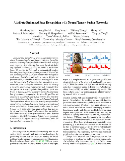
Attribute-Enhanced Face Recognition with Neural Tensor Fusion Networks Guosheng Hu1Yang Hua1,2Yang Yuan1Zhihong Zhang3Zheng Lu1 Sankha S.Mukherjee1Timothy M.Hospedales4Neil M.Robertson1,2Yongxin Yang5,61AnyVision2Queen’s University Belfast3Xiamen University 4The University of Edinburgh5Queen Mary University of London6Yang’s Accounting Consultancy Ltd {guosheng.hu,yang.hua,yuany,steven,rick}@,N.Robertson@ zhihong@,t.hospedales@,yongxin@yang.acAbstractDeep learning has achieved great success in face recog-nition,however deep-learned features still have limited in-variance to strong intra-personal variations such as large pose changes.It is observed that some facial attributes (e.g.eyebrow thickness,gender)are robust to such varia-tions.We present thefirst work to systematically explore how the fusion of face recognition features(FRF)and fa-cial attribute features(FAF)can enhance face recognition performance in various challenging scenarios.Despite the promise of FAF,wefind that in practice existing fusion meth-ods fail to leverage FAF to boost face recognition perfor-mance in some challenging scenarios.Thus,we develop a powerful tensor-based framework which formulates fea-ture fusion as a tensor optimisation problem.It is non-trivial to directly optimise this tensor due to the large num-ber of parameters to optimise.To solve this problem,we establish a theoretical equivalence between low-rank ten-sor optimisation and a two-stream gated neural network. This equivalence allows tractable learning using standard neural network optimisation tools,leading to accurate and stable optimisation.Experimental results show the fused feature works better than individual features,thus proving for thefirst time that facial attributes aid face recognition. We achieve state-of-the-art performance on three popular databases:MultiPIE(cross pose,lighting and expression), CASIA NIR-VIS2.0(cross-modality environment)and LFW (uncontrolled environment).1.IntroductionFace recognition has advanced dramatically with the ad-vent of bigger datasets,and improved methodologies for generating features that are variant to identity but invari-ant to covariates such as pose,expression and illumination. Deep learning methodologies[41,40,42,32]have proven particularly effective recently,thanks to end-to-endrepre-Figure1:A sample attribute list is given(col.1)which per-tains to the images of the same individual at different poses (col.2).While the similarity scores for each dimension vary in the face recognition feature(FRF)set(col.3),the face at-tribute feature(FAF)set(col.4)remains very similar.The fused features(col.5)are more similar and a higher similar-ity score(0.89)is achieved.sentation learning with a discriminative face recognition ob-jective.Nevertheless,the resulting features still show im-perfect invariance to the strong intra-personal variations in real-world scenarios.We observe that facial attributes pro-vide a robust invariant cue in such challenging scenarios.For example gender and ethnicity are likely to be invariant to pose and expression,while eyebrow thickness may be invariant to lighting and resolution.Overall,face recogni-tion features(FRF)are very discriminative but less robust;while facial attribute features(FAF)are robust but less dis-criminative.Thus these two features are potentially com-plementary,if a suitable fusion method can be devised.To the best of our knowledge,we are thefirst to systematically explore the fusion of FAF and FRF in various face recog-nition scenarios.We empirically show that this fusion can greatly enhance face recognition performance.Though facial attributes are an important cue for face recognition,in practice,wefind the existing fusion meth-ods including early(feature)or late(score)fusion cannot reliably improve the performance[34].In particular,while 1offering some robustness,FAF is generally less discrimina-tive than FRF.Existing methods cannot synergistically fuse such asymmetric features,and usually lead to worse perfor-mance than achieved by the stronger feature(FRF)only.In this work,we propose a novel tensor-based fusion frame-work that is uniquely capable of fusing the very asymmet-ric FAF and FRF.Our framework provides a more powerful and robust fusion approach than existing strategies by learn-ing from all interactions between the two feature views.To train the tensor in a tractable way given the large number of required parameters,we formulate the optimisation with an identity-supervised objective by constraining the tensor to have a low-rank form.We establish an equivalence be-tween this low-rank tensor and a two-stream gated neural network.Given this equivalence,the proposed tensor is eas-ily optimised with standard deep neural network toolboxes. Our technical contributions are:•It is thefirst work to systematically investigate and ver-ify that facial attributes are an important cue in various face recognition scenarios.In particular,we investi-gate face recognition with extreme pose variations,i.e.±90◦from frontal,showing that attributes are impor-tant for performance enhancement.•A rich tensor-based fusion framework is proposed.We show the low-rank Tucker-decomposition of this tensor-based fusion has an equivalent Gated Two-stream Neural Network(GTNN),allowing easy yet effective optimisation by neural network learning.In addition,we bring insights from neural networks into thefield of tensor optimisation.The code is available:https:///yanghuadr/ Neural-Tensor-Fusion-Network•We achieve state-of-the-art face recognition perfor-mance using the fusion of face(newly designed‘Lean-Face’deep learning feature)and attribute-based fea-tures on three popular databases:MultiPIE(controlled environment),CASIA NIR-VIS2.0(cross-modality environment)and LFW(uncontrolled environment).2.Related WorkFace Recognition.The face representation(feature)is the most important component in contemporary face recog-nition system.There are two types:hand-crafted and deep learning features.Widely used hand-crafted face descriptors include Local Binary Pattern(LBP)[26],Gaborfilters[23],-pared to pixel values,these features are variant to identity and relatively invariant to intra-personal variations,and thus they achieve promising performance in controlled environ-ments.However,they perform less well on face recognition in uncontrolled environments(FRUE).There are two main routes to improve FRUE performance with hand-crafted features,one is to use very high dimensional features(dense sampling features)[5]and the other is to enhance the fea-tures with downstream metric learning.Unlike hand-crafted features where(in)variances are en-gineered,deep learning features learn the(in)variances from data.Recently,convolutional neural networks(CNNs) achieved impressive results on FRUE.DeepFace[44],a carefully designed8-layer CNN,is an early landmark method.Another well-known line of work is DeepID[41] and its variants DeepID2[40],DeepID2+[42].The DeepID family uses an ensemble of many small CNNs trained in-dependently using different facial patches to improve the performance.In addition,some CNNs originally designed for object recognition,such as VGGNet[38]and Incep-tion[43],were also used for face recognition[29,32].Most recently,a center loss[47]is introduced to learn more dis-criminative features.Facial Attribute Recognition.Facial attribute recog-nition(FAR)is also well studied.A notable early study[21] extracted carefully designed hand-crafted features includ-ing aggregations of colour spaces and image gradients,be-fore training an independent SVM to detect each attribute. As for face recognition,deep learning features now outper-form hand-crafted features for FAR.In[24],face detection and attribute recognition CNNs are carefully designed,and the output of the face detection network is fed into the at-tribute network.An alternative to purpose designing CNNs for FAR is tofine-tune networks intended for object recog-nition[56,57].From a representation learning perspective, the features supporting different attribute detections may be shared,leading some studies to investigate multi-task learn-ing facial attributes[55,30].Since different facial attributes have different prevalence,the multi-label/multi-task learn-ing suffers from label-imbalance,which[30]addresses us-ing a mixed objective optimization network(MOON). Face Recognition using Facial Attributes.Detected facial attributes can be applied directly to authentication. Facial attributes have been applied to enhance face verifica-tion,primarily in the case of cross-modal matching,byfil-tering[19,54](requiring potential FRF matches to have the correct gender,for example),model switching[18],or ag-gregation with conventional features[27,17].[21]defines 65facial attributes and proposes binary attribute classifiers to predict their presence or absence.The vector of attribute classifier scores can be used for face recognition.There has been little work on attribute-enhanced face recognition in the context of deep learning.One of the few exploits CNN-based attribute features for authentication on mobile devices [31].Local facial patches are fed into carefully designed CNNs to predict different attributes.After CNN training, SVMs are trained for attribute recognition,and the vector of SVM scores provide the new feature for face verification.Fusion Methods.Existing fusion approaches can be classified into feature-level(early fusion)and score-level (late fusion).Score-level fusion is to fuse the similarity scores after computation based on each view either by sim-ple averaging[37]or stacking another classifier[48,37]. Feature-level fusion can be achieved by either simple fea-ture aggregation or subspace learning.For aggregation ap-proaches,fusion is usually performed by simply element wise averaging or product(the dimension of features have to be the same)or concatenation[28].For subspace learn-ing approaches,the features arefirst concatenated,then the concatenated feature is projected to a subspace,in which the features should better complement each other.These sub-space approaches can be unsupervised or supervised.Un-supervised fusion does not use the identity(label)informa-tion to learn the subspace,such as Canonical Correlational Analysis(CCA)[35]and Bilinear Models(BLM)[45].In comparison,supervised fusion uses the identity information such as Linear Discriminant Analysis(LDA)[3]and Local-ity Preserving Projections(LPP)[9].Neural Tensor Methods.Learning tensor-based compu-tations within neural networks has been studied for full[39] and decomposed[16,52,51]tensors.However,aside from differing applications and objectives,the key difference is that we establish a novel equivalence between a rich Tucker [46]decomposed low-rank fusion tensor,and a gated two-stream neural network.This allows us achieve expressive fusion,while maintaining tractable computation and a small number of parameters;and crucially permits easy optimisa-tion of the fusion tensor through standard toolboxes. Motivation.Facial attribute features(FAF)and face recognition features(FRF)are complementary.However in practice,wefind that existing fusion methods often can-not effectively combine these asymmetric features so as to improve performance.This motivates us to design a more powerful fusion method,as detailed in Section3.Based on our neural tensor fusion method,in Section5we system-atically explore the fusion of FAF and FRF in various face recognition environments,showing that FAF can greatly en-hance recognition performance.3.Fusing attribute and recognition featuresIn this section we present our strategy for fusing FAF and FRF.Our goal is to input FAF and FRF and output the fused discriminative feature.The proposed fusion method we present here performs significantly better than the exist-ing ones introduced in Section2.In this section,we detail our tensor-based fusion strategy.3.1.ModellingSingle Feature.We start from a standard multi-class clas-sification problem setting:assume we have M instances, and for each we extract a D-dimensional feature vector(the FRF)as{x(i)}M i=1.The label space contains C unique classes(person identities),so each instance is associated with a corresponding C-dimensional one-hot encoding la-bel vector{y(i)}M i=1.Assuming a linear model W the pre-dictionˆy(i)is produced by the dot-product of input x(i)and the model W,ˆy(i)=x(i)T W.(1) Multiple Feature.Suppose that apart from the D-dimensional FRF vector,we can also obtain an instance-wise B-dimensional facial attribute feature z(i).Then the input for the i th instance is a pair:{x(i),z(i)}.A simple ap-proach is to redefine x(i):=[x(i),z(i)],and directly apply Eq.(1),thus modelling weights for both FRF and FAF fea-tures.Here we propose instead a non-linear fusion method via the following formulationˆy(i)=W×1x(i)×3z(i)(2) where W is the fusion model parameters in the form of a third-order tensor of size D×C×B.Notation×is the tensor dot product(also known as tensor contraction)and the left-subscript of x and z indicates at which axis the ten-sor dot product operates.With Eq.(2),the optimisation problem is formulated as:minW1MMi=1W×1x(i)×3z(i),y(i)(3)where (·,·)is a loss function.This trains tensor W to fuse FRF and FAF features so that identity is correctly predicted.3.2.OptimisationThe proposed tensor W provides a rich fusion model. However,compared with W,W is B times larger(D×C vs D×C×B)because of the introduction of B-dimensional attribute vector.It is also almost B times larger than train-ing a matrix W on the concatenation[x(i),z(i)].It is there-fore problematic to directly optimise Eq.(3)because the large number of parameters of W makes training slow and leads to overfitting.To address this we propose a tensor de-composition technique and a neural network architecture to solve an equivalent optimisation problem in the following two subsections.3.2.1Tucker Decomposition for Feature FusionTo reduce the number of parameters of W,we place a struc-tural constraint on W.Motivated by the famous Tucker de-composition[46]for tensors,we assume that W is synthe-sised fromW=S×1U(D)×2U(C)×3U(B).(4) Here S is a third order tensor of size K D×K C×K B, U(D)is a matrix of size K D×D,U(C)is a matrix of sizeK C×C,and U(B)is a matrix of size K B×B.By restricting K D D,K C C,and K B B,we can effectively reduce the number of parameters from(D×C×B)to (K D×K C×K B+K D×D+K C×C+K B×B)if we learn{S,U(D),U(C),U(B)}instead of W.When W is needed for making the predictions,we can always synthesise it from those four small factors.In the context of tensor decomposition,(K D,K C,K B)is usually called the tensor’s rank,as an analogous concept to the rank of a matrix in matrix decomposition.Note that,despite of the existence of other tensor de-composition choices,Tucker decomposition offers a greater flexibility in terms of modelling because we have three hyper-parameters K D,K C,K B corresponding to the axes of the tensor.In contrast,the other famous decomposition, CP[10]has one hyper-parameter K for all axes of tensor.By substituting Eq.(4)into Eq.(2),we haveˆy(i)=W×1x(i)×3z(i)=S×1U(D)×2U(C)×3U(B)×1x(i)×3z(i)(5) Through some re-arrangement,Eq.(5)can be simplified as ˆy(i)=S×1(U(D)x(i))×2U(C)×3(U(B)z(i))(6) Furthermore,we can rewrite Eq.(6)as,ˆy(i)=((U(D)x(i))⊗(U(B)z(i)))S T(2)fused featureU(C)(7)where⊗is Kronecker product.Since U(D)x(i)and U(B)B(i)result in K D and K B dimensional vectors re-spectively,(U(D)x(i))⊗(U(B)z(i))produces a K D K B vector.S(2)is the mode-2unfolding of S which is aK C×K D K B matrix,and its transpose S T(2)is a matrix ofsize K D K B×K C.The Fused Feature.From Eq.(7),the explicit fused representation of face recognition(x(i))and facial at-tribute(z(i))features can be achieved.The fused feature ((U(D)x(i))⊗(U(B)z(i)))S T(2),is a vector of the dimen-sionality K C.And matrix U(C)has the role of“clas-sifier”given this fused feature.Given{x(i),z(i),y(i)}, the matrices{U(D),U(B),U(C)}and tensor S are com-puted(learned)during model optimisation(training).Dur-ing testing,the predictionˆy(i)is achieved with the learned {U(D),U(B),U(C),S}and two test features{x(i),z(i)} following Eq.(7).3.2.2Gated Two-stream Neural Network(GTNN)A key advantage of reformulating Eq.(5)into Eq.(7)is that we can nowfind a neural network architecture that does ex-actly the computation of Eq.(7),which would not be obvi-ous if we stopped at Eq.(5).Before presenting thisneural Figure2:Gated two-stream neural network to implement low-rank tensor-based fusion.The architecture computes Eq.(7),with the Tucker decomposition in Eq.(4).The network is identity-supervised at train time,and feature in the fusion layer used as representation for verification. network,we need to introduce a new deterministic layer(i.e. without any learnable parameters).Kronecker Product Layer takes two arbitrary-length in-put vectors{u,v}where u=[u1,u2,···,u P]and v=[v1,v2,···,v Q],then outputs a vector of length P Q as[u1v1,u1v2,···,u1v Q,u2v1,···,u P v Q].Using the introduced Kronecker layer,Fig.2shows the neural network that computes Eq.(7).That is,the neural network that performs recognition using tensor-based fu-sion of two features(such as FAF and FRF),based on the low-rank assumption in Eq.(4).We denote this architecture as a Gated Two-stream Neural Network(GTNN),because it takes two streams of inputs,and it performs gating[36] (multiplicative)operations on them.The GTNN is trained in a supervised fashion to predict identity.In this work,we use a multitask loss:softmax loss and center loss[47]for joint training.The fused feature in the viewpoint of GTNN is the output of penultimate layer, which is of dimensionality K c.So far,the advantage of using GTNN is obvious.Direct use of Eq.(5)or Eq.(7)requires manual derivation and im-plementation of an optimiser which is non-trivial even for decomposed matrices(2d-tensors)[20].In contrast,GTNN is easily implemented with modern deep learning packages where auto-differentiation and gradient-based optimisation is handled robustly and automatically.3.3.DiscussionCompared with the fusion methods introduced in Sec-tion2,we summarise the advantages of our tensor-based fusion method as follows:Figure3:LeanFace.‘C’is a group of convolutional layers.Stage1:64@5×5(64feature maps are sliced to two groups of32ones, which are fed into maxout function.);Stage2:64@3×3,64@3×3,128@3×3,128@3×3;Stage3:196@3×3,196@3×3, 256@3×3,256@3×3,320@3×3,320@3×3;Stage4:512@3×3,512@3×3,512@3×3,512@3×3;Stage5:640@ 5×5,640@5×5.‘P’stands for2×2max pooling.The strides for the convolutional and pooling layers are1and2,respectively.‘FC’is a fully-connected layer of256D.High Order Non-Linearity.Unlike linear methods based on averaging,concatenation,linear subspace learning [8,27],or LDA[3],our fusion method is non-linear,which is more powerful to model complex problems.Further-more,comparing with otherfirst-order non-linear methods based on element-wise combinations only[28],our method is higher order:it accounts for all interactions between each pair of feature channels in both views.Thanks to the low-rank modelling,our method achieves such powerful non-linear fusion with few parameters and thus it is robust to overfitting.Scalability.Big datasets are required for state-of-the-art face representation learning.Because we establish the equivalence between tensor factorisation and gated neural network architecture,our method is scalable to big-data through efficient mini-batch SGD-based learning.In con-trast,kernel-based non-linear methods,such as Kernel LDA [34]and multi-kernel SVM[17],are restricted to small data due to their O(N2)computation cost.At runtime,our method only requires a simple feed-forward pass and hence it is also favourable compared to kernel methods. Supervised method.GTNN isflexibly supervised by any desired neural network loss function.For example,the fusion method can be trained with losses known to be ef-fective for face representation learning:identity-supervised softmax,and centre-loss[47].Alternative methods are ei-ther unsupervised[8,27],constrained in the types of super-vision they can exploit[3,17],or only stack scores rather than improving a learned representation[48,37].There-fore,they are relatively ineffective at learning how to com-bine the two-source information in a task-specific way. Extensibility.Our GTNN naturally can be extended to deeper architectures.For example,the pre-extracted fea-tures,i.e.,x and z in Fig.2,can be replaced by two full-sized CNNs without any modification.Therefore,poten-tially,our methods can be integrated into an end-to-end framework.4.Integration with CNNs:architectureIn this section,we introduce the CNN architectures used for face recognition(LeanFace)designed by ourselves and facial attribute recognition(AttNet)introduced by[50,30]. LeanFace.Unlike general object recognition,face recognition has to capture very subtle difference between people.Motivated by thefine-grain object recognition in [4],we also use a large number of convolutional layers at early stage to capture the subtle low level and mid-level in-formation.Our activation function is maxout,which shows better performance than its competitors[50].Joint supervi-sion of softmax loss and center loss[47]is used for training. The architecture is summarised in Fig.3.AttNet.To detect facial attributes,our AttNet uses the ar-chitecture of Lighten CNN[50]to represent a face.Specifi-cally,AttNet consists of5conv-activation-pooling units fol-lowed by a256D fully connected layer.The number of con-volutional kernels is explained in[50].The activation func-tion is Max-Feature-Map[50]which is a variant of maxout. We use the loss function MOON[30],which is a multi-task loss for(1)attribute classification and(2)domain adaptive data balance.In[24],an ontology of40facial attributes are defined.We remove attributes which do not characterise a specific person,e.g.,‘wear glasses’and‘smiling’,leaving 17attributes in total.Once each network is trained,the features extracted from the penultimate fully-connected layers of LeanFace(256D) and AttNet(256D)are extracted as x and z,and input to GTNN for fusion and then face recognition.5.ExperimentsWefirst introduce the implementation details of our GTNN method.In Section5.1,we conduct experiments on MultiPIE[7]to show that facial attributes by means of our GTNN method can play an important role on improv-Table1:Network training detailsImage size BatchsizeLR1DF2EpochTraintimeLeanFace128x1282560.0010.15491hAttNet0.050.8993h1Learning rate(LR)2Learning rate drop factor(DF).ing face recognition performance in the presence of pose, illumination and expression,respectively.Then,we com-pare our GTNN method with other fusion methods on CA-SIA NIR-VIS2.0database[22]in Section5.2and LFW database[12]in Section5.3,respectively. Implementation Details.In this study,three networks (LeanFace,AttNet and GTNN)are discussed.LeanFace and AttNet are implemented using MXNet[6]and GTNN uses TensorFlow[1].We use around6M training face thumbnails covering62K different identities to train Lean-Face,which has no overlapping with all the test databases. AttNet is trained using CelebA[24]database.The input of GTNN is two256D features from bottleneck layers(i.e., fully connected layers before prediction layers)of LeanFace and AttNet.The setting of main parameters are shown in Table1.Note that the learning rates drop when the loss stops decreasing.Specifically,the learning rates change4 and2times for LeanFace and AttNet respectively.Dur-ing test,LeanFace and AttNet take around2.9ms and3.2ms to extract feature from one input image and GTNN takes around2.1ms to fuse one pair of LeanFace and AttNet fea-ture using a GTX1080Graphics Card.5.1.Multi-PIE DatabaseMulti-PIE database[7]contains more than750,000im-ages of337people recorded in4sessions under diverse pose,illumination and expression variations.It is an ideal testbed to investigate if facial attribute features(FAF) complement face recognition features(FRF)including tra-ditional hand-crafted(LBP)and deeply learned features (LeanFace)to improve the face recognition performance–particularly across extreme pose variation.Settings.We conduct three experiments to investigate pose-,illumination-and expression-invariant face recogni-tion.Pose:Uses images across4sessions with pose vari-ations only(i.e.,neutral lighting and expression).It covers pose with yaw ranging from left90◦to right90◦.In com-parison,most of the existing works only evaluate perfor-mance on poses with yaw range(-45◦,+45◦).Illumination: Uses images with20different illumination conditions(i.e., frontal pose and neutral expression).Expression:Uses im-ages with7different expression variations(i.e.,frontal pose and neutral illumination).The training sets of all settings consist of the images from thefirst200subjects and the re-maining137subjects for testing.Following[59,14],in the test set,frontal images with neural illumination and expres-sion from the earliest session work as gallery,and the others are probes.Pose.Table2shows the pose-robust face recognition (PRFR)performance.Clearly,the fusion of FRF and FAF, namely GTNN(LBP,AttNet)and GTNN(LeanFace,At-tNet),works much better than using FRF only,showing the complementary power of facial features to face recognition features.Not surprisingly,the performance of both LBP and LeanFace features drop greatly under extreme poses,as pose variation is a major factor challenging face recognition performance.In contrast,with GTNN-based fusion,FAF can be used to improve both classic(LBP)and deep(Lean-Face)FRF features effectively under this circumstance,for example,LBP(1.3%)vs GTNN(LBP,AttNet)(16.3%), LeanFace(72.0%)vs GTNN(LeanFace,AttNet)(78.3%) under yaw angel−90◦.It is noteworthy that despite their highly asymmetric strength,GTNN is able to effectively fuse FAF and FRF.This is elaborately studied in more detail in Sections5.2-5.3.Compared with state-of-the-art methods[14,59,11,58, 15]in terms of(-45◦,+45◦),LeanFace achieves better per-formance due to its big training data and the strong gener-alisation capacity of deep learning.In Table2,2D meth-ods[14,59,15]trained models using the MultiPIE images, therefore,they are difficult to generalise to images under poses which do not appear in MultiPIE database.3D meth-ods[11,58]highly depend on accurate2D landmarks for 3D-2D modellingfitting.However,it is hard to accurately detect such landmarks under larger poses,limiting the ap-plications of3D methods.Illumination and expression.Illumination-and expression-robust face recognition(IRFR and ERFR)are also challenging research topics.LBP is the most widely used handcrafted features for IRFR[2]and ERFR[33].To investigate the helpfulness of facial attributes,experiments of IRFR and ERFR are conducted using LBP and Lean-Face features.In Table3,GTNN(LBP,AttNet)signifi-cantly outperforms LBP,80.3%vs57.5%(IRFR),77.5% vs71.7%(ERFR),showing the great value of combining fa-cial attributes with hand-crafted features.Attributes such as the shape of eyebrows are illumination invariant and others, e.g.,gender,are expression invariant.In contrast,LeanFace feature is already very discriminative,saturating the perfor-mance on the test set.So there is little room for fusion of AttrNet to provide benefit.5.2.CASIA NIR-VIS2.0DatabaseThe CASIA NIR-VIS2.0face database[22]is the largest public face database across near-infrared(NIR)images and visible RGB(VIS)images.It is a typical cross-modality or heterogeneous face recognition problem because the gallery and probe images are from two different spectra.The。

doi:10.19677/j.issn.1004-7964.2024.01.005基于改进YOLOv5的皮革抓取点识别及定位金光，任工昌*，桓源，洪杰（陕西科技大学机电工程学院，陕西西安710021）摘要：为实现机器人对皮革抓取点的精确定位，文章通过改进YOLOv5算法，引入coordinate attention 注意力机制到Backbone 层中，用Focal-EIOU Loss 对CIOU Loss 进行替换来设置不同梯度，从而实现了对皮革抓取点快速精准的识别和定位。

利用目标边界框回归公式获取皮革抓点的定位坐标，经过坐标系转换获得待抓取点的三维坐标，采用Intel RealSense D435i 深度相机对皮革抓取点进行定位实验。

实验结果表明：与Faster R-CNN 算法和原始YOLOv5算法对比，识别实验中改进YOLOv5算法的准确率分别提升了6.9%和2.63%，召回率分别提升了8.39%和2.63%，mAP 分别提升了8.13%和0.21%；定位实验中改进YOLOv5算法的误差平均值分别下降了0.033m 和0.007m，误差比平均值分别下降了2.233%和0.476%。

关键词:皮革；抓取点定位；机器视觉；YOLOv5；CA 注意力机制中图分类号:TP 391文献标志码:AGrab Point Identification and Localization of Leather based onImproved YOLOv5(College of Mechanical and Electrical Engineering,Shaanxi University of Science and Technology,Xi ’an 710021,China)Abstract:In order to achieve precise localization of leather grasping points by robots,this study proposed an improved approach based on the YOLOv5algorithm.The methodology involved the integration of the coordinate attention mechanism into the Backbone layer and the replacement of the CIOU Loss with the Focal-EIOU Loss to enable different gradients and enhance the rapid and accurate recognition and localization of leather grasping points.The positioning coordinates of the leather grasping points were obtained by using the target bounding box regression formula,followed by the coordinate system conversion to obtain the three-dimensional coordinates of the target grasping points.The experimental positioning of leather grasping points was conducted by using the Intel RealSense D435i depth camera.Experimental results demonstrate the significant improvements over the Faster R -CNN algorithm and the original YOLOv5algorithm.The improved YOLOv5algorithm exhibited an accuracy enhancement of 6.9%and 2.63%,a recall improvement of 8.39%and 2.63%,and an mAP improvement of 8.13%and 0.21%in recognition experiments,respectively.Similarly,in the positioning experiments,the improved YOLOv5algorithm demonstrated a decrease in average error values of 0.033m and 0.007m,and a decrease in error ratio average values of 2.233%and 0.476%.Key words:leather;grab point positioning;machine vision;YOLOv5;coordinate attention收稿日期：2023-06-09修回日期：2023-07-08接受日期：2023-07-12基金项目：陕西省重点研发计划资助项目（2022GY-250）；西安市科技计划项目（23ZDCYJSGG0016-2022）第一作者简介：金光（1996-），男，硕士研究生，主要研究方向为机器视觉,深度学习。

第37卷第1期湖南理工学院学报(自然科学版)V ol. 37 No. 1 2024年3月 Journal of Hunan Institute of Science and Technology (Natural Sciences) Mar. 2024引入稳定学习的多中心脑磁共振影像统计分类方法研究杨勃, 钟志锴(湖南理工学院信息科学与工程学院, 湖南岳阳 414006)摘要:针对现有统计分析方法在多中心统计分类任务上缺乏稳定性的问题, 提出一种引入稳定学习的多中心脑磁共振影像的统计分类方法. 该方法使用多层3D卷积神经网络作为骨干结构, 并引入稳定学习旁路结构调节卷积网络习得特征的稳定性. 在稳定学习旁路中, 首先使用随机傅里叶变换获取卷积网络特征的多路随机序列, 然后通过学习和优化批次样本采样权重以获取卷积网络特征之间的独立性, 从而改善跨中心分类泛化性. 最后, 在公开数据库FCP中的3中心脑影像数据集上进行跨中心性别分类实验. 实验结果表明, 与基准卷积网络相比, 引入稳定学习的卷积网络具有更高的跨中心分类正确率, 有效提高了跨中心泛化性和多中心统计分类的稳定性.关键词:多中心脑磁共振影像分析; 卷积神经网络; 稳定学习; 跨中心泛化中图分类号: TP183 文章编号: 1672-5298(2024)01-0015-05 Research on a Classification Approach for Multi-site Brain Magnetic Resonance Imaging Analysis byIntroducing Stable LearningYANG Bo, ZHONG Zhikai(School of Information Science and Engineering, Hunan Institute of Science and Technology, Yueyang 414006, China) Abstract: Aiming at the lack of stability of existing statistical analysis methods suitable for single site tasks in a multi-site setting, a statistical classification approach integrating stable learning for multi-site brain magnetic resonance imaging(MRI) analysis tasks was proposed. In the proposed approach, a multi-layer 3-dimensional convolutional neural network(3D CNN) was used as the backbone structure, while a stable learning module used for improving the stability of features learning by CNN was integrated as bypassing structure. In the stable learning module, the random Fourier transform was firstly used to obtain the random sequences of CNN features, and then the independence between different sequences was obtained by optimizing sampling weights of every sample batch and improving the cross-site generalization. Finally, a cross-site gender classification experiment was conducted on the 3 brain MRI data site from the publicly available database FCP. The experimental results show that compared with the basic CNN, the CNN with stable learning has a higher accuracy in cross-site classification, and effectively improves the stability of cross-center generalization and multi-center statistical classification.Key words: multi-site brain MRI analysis; convolutional neural network; stable learning; cross-site generalization0 引言经典机器学习方法使用训练数据集来训练模型, 然后使用训练好的模型对新数据进行预测. 确保该训练—预测流程的有效性, 主要基于两点[1]: 一是理论上满足独立同分布假设, 即训练数据和新数据均独立采样自同一统计分布; 二是训练数据量要充分, 能够准确描述该统计分布.在大量实际应用中, 收集到的数据往往来自不同数据域, 不满足独立同分布假设, 导致经典机器学习方法在此场景下性能显著退化, 在某一个域中训练得到的模型完全无法迁移到其他域的数据上, 跨域泛化性差[2]. 磁共振影像(Magnetic Resonance Imaging, MRI)分析领域也同样存在此类问题. 为增大数据量以获得更优的训练效果, 单中心脑MRI分析已逐渐发展到多中心脑MRI分析. 虽然多中心影像数据量显著增收稿日期: 2023-06-19基金项目:湖南省研究生科研创新项目(CX20221231,YCX2023A50); 湖南省自然科学基金项目“面向小样本脑磁共振影像分析的数据生成技术与深度学习方法研究”(2024JJ7208)作者简介: 杨勃, 男, 博士, 教授. 主要研究方向: 机器学习、脑影像分析16 湖南理工学院学报(自然科学版) 第37卷长, 但由于存在机器参数、被试生理参数等诸多不同, 不同中心的数据无法满足独立同分布假设, 导致多中心统计分析表现出较差的稳定性[3,4].为提升多域分析的稳定性, 近年来机器学习理论研究从因果分析角度提出一系列基于线性无关特征采样的稳定预测方法[5,6], 并在低维数据上取得了一定效果, 初步展现出在多域分析上的巨大潜力. Zhang等[7]在此基础上提出稳定学习方法, 扩展了以前的线性框架, 以纳入深度模型. 由于在深度模型中获得的复杂非线性特征之间的依赖关系比线性情况下更难测量和消除[8,9], 因此稳定学习采用了一种基于随机傅里叶特征(Random Fourier Features, RFF)[10]的非线性特征去相关方法; 同时, 为了适应现代深度模型, 还专门设计了一种全局关联的保存和重新加载机制, 以减少训练大规模数据时的存储和计算成本. 相关实验表明, 稳定学习结合深度学习在高维图像识别任务上表现出较好的稳定性[7].本文尝试将稳定学习引入多中心脑MRI 的统计分类任务中, 将稳定学习与3D CNN 结合, 解决跨中心泛化性问题, 提高多中心分类稳定性. 首先介绍本研究设计的融合稳定学习的3D CNN 网络架构; 然后介绍稳定学习特征独立性最大化准则; 最后与基准3D CNN 分别在公开数据集FCP 中的3中心脑MRI 数据集上进行对比分类实验. 实验结果表明, 引入稳定学习的卷积网络具有更高的跨中心分类正确率, 有效提高了多中心脑MRI 统计分类的稳定性.1 融合稳定学习的3D CNN 架构设计融合稳定学习的3D CNN 总体架构设计如图1所示. 首先使用3D CNN 提取脑MRI 的3D 特征, 再将特征分别输出至稳定学习旁路和分类器主路进行训练. 稳定学习旁路使用随机傅里叶变换模块提取3D特征的多路RFF 特征, 然后使用样本加权解相关模块(Learning Sample Weighting for Decorrelation, LSWD)优化样本采样权重. 最后使用样本权重对分类器的预测损失进行加权, 以加权损失最小化为优化目标进行反向传播.图1 融合稳定学习的3D CNN 总体架构设计2 特征独立性最大化2.1 基于随机傅里叶变换的随机变量独立性判定设X 、Y 为两个随机变量, ()X f X 、()Y f Y 、(,)f X Y 分别表示X 的概率密度、Y 的概率密度以及X 和Y 的联合概率密度, 若满足(,)()()X Y f X Y f X f Y =,则称随机变量X 、Y 相互独立.当X 、Y 均服从高斯分布时, 统计独立性等价于统计不相关, 即Conv (,)((())(()))()()()0X Y E X E x Y E Y E XY E X E Y =--=-=,其中Conv (,)⋅⋅为两随机变量之间的协方差, ()E ⋅为随机变量的期望.第1期 杨 勃, 等: 引入稳定学习的多中心脑磁共振影像统计分类方法研究 17在本文深度神经网络中, 随机变量,X Y 就是脑MRI 的3D 特征变量. 设有n 个训练样本, 可将其视为对随机变量,X Y 分别进行了n 次采样, 获得了对应的随机序列12(,,,)n X x x x = 和12(,,,)nY y y y = . 可使用随机序列之间的协方差进行无偏估计:Conv 111()111,1n n n i j i j i j j X Y x x y y n n n ===⎛⎫⎛⎫=-- ⎪ ⎪-⎝⎭⎝⎭∑∑∑ . 需要指出的是, 若,X Y 不服从高斯分布, 则Conv0(),X Y = 不能作为变量独立性判定准则. 文[9]指出, 此情形下可将随机序列,X Y 转换为k 个随机傅里叶变换序列{RFF },){RFF }()(i i k i i kX Y ≤≤后再使用协方差进行判定.随机傅里叶变换公式为RFF ,)()(s i i i X X ωφ+ ~(0,1),i N ω~Uniform(0,2π),iφi <∞. 其中随机频率i ω从标准正态分布中采样得到, 随机相位i φ从0~2π之间的均匀分布中采样得到.通过随机傅里叶变换可获得如下两个随机矩阵RFF(),RFF()n k XY ⨯∈ : 1212RFF()(RFF ,RFF ,,RFF ),R .()())FF()(F ()RF ,RF ,()(F ,RFF ())k kX X X X Y Y Y Y == 计算这两个随机矩阵的协方差矩阵:Conv T111111(((RFF ),RF ()()()(F())RFF RFF RFF RFF 1)n n n i j i j i j j X Y X X Y Y n n n ===⎡⎤=--⎢⎣⎥-⎣⎦⎡⎤⎢⎥⎦∑∑∑ . 若||Conv 2(RFF(),RFF())||0,F X Y = 则可判定随机变量,X Y 相互独立. 本文参照文[6]建议, 固定5k =.2.2 基于样本加权的特征独立性最大化在融合稳定学习的深度神经网络中, 通过LSWD 模块优化样本权重并最大化特征之间的独立性, 优化准则如下:,1,j |arg min |()m i j i L =<=∑w Conv (RFF(w ⨀i Q ), RFF(w ⨀2))||j F Q , T s.t.,n >=0w w e .其中1n i ⨯∈ Q 为网络输出的第i 个特征序列, ⨀为Hamard 乘积运算, 1n ⨯∈ w 为n 个样本的权重, e 为全1向量. 上述优化准则, 可使得深度神经网络输出特征两两之间相互独立.3 实验结果与分析3.1 实验数据与预处理实验数据来自网上公共数据库1000功能连接组计划(1000 Functional Connectomes Project, FCP). 该公共数据库收集了35个中心合计1355名被试的脑MRI 数据. 本实验使用了FCP 中3个中心的数据集, 分别为:北京(Beijing)、剑桥(Cambridge)和国际医学会议(ICBM)[11], 主要任务是使用其中的3D 脑结构MRI 数据完成性别分类. 其中, Beijing 数据集包含被试样本140个(男性70个/女性70个), Cambridge 数据集包含被试样本198个(男性75个/女性123个), ICBM 数据集包含被试样本86个(男性41个/女性45个).在Matlab 2015中使用SPM8工具包对原始脑结构MRI 数据进行如下数据预处理:第1步 脑影像颅骨剥离;第2步 分割去颅骨脑影像为灰质、白质和脑脊液3部分(本实验仅使用灰质数据);第3步 标准化预处理, 将脑影像统一配准到MNI(Montreal Neurological Institute)模版空间;第4步 去噪与平滑预处理, 使用高斯平滑方法平滑标准化灰质影像.预处理后, 最终得到尺寸大小为121×145×121的3D 结构影像.18 湖南理工学院学报(自然科学版) 第37卷此外, 为减少后续计算量, 通过尺度缩放操作将预处理后的3D 结构影像尺寸进一步缩小至64×64×64.然后使用Z-Score 标准化方法对每个中心的数据分别进行中心偏差校正.3.2 分类器参数设置分别测试了基准3D CNN 和融合稳定学习的3D CNN 的多中心脑MRI 分类性能. 其中3D CNN 架构部分,两种分类器均采用同样的网络架构和参数, 具体如下.网络层数设计为5层, 每层包含2个3D 卷积操作(with padding), 2个ReLU 非线性映射操作和1个3D maxpooling 操作(每层窗宽均为2). 其中, 第1层卷积核尺寸为7×7×7, 第2~5层卷积核尺寸均为3×3×3, 1~5层输出通道大小分别为32、64、128、256、512.使用Pytorch 1.12.0平台搭建网络. 训练时, 初始学习率固定为0.001, 使用Adam 优化器进行训练,batchsize 固定为128(男女样本各64个).3.3 跨中心性别分类实验采用域泛化实验设置LOSO(Leave One Site Out)来测试不同分类器的跨中心脑MRI 分类的泛化能力, 即留一个中心数据作为测试数据, 其他中心数据作为训练数据. 在训练过程中, 确保用于测试的中心数据完全隔离. 实验重复三次, 使用不同的随机种子, 取平均值作为最终结果. 跨中心分类平均正确率见表1.表1 跨中心分类平均正确率(%)对比方法 测试中心 总体平均分类正确率(Cambridge, ICBM)-Beijing (Beijing, ICBM)-Cambridge (Cambridge, Beijing)-ICBMbase 75.76 73.91 72.48 74.05stable 78.11 75.59 75.97 76.56* base: 基准3D CNN; stable: 融合稳定学习的3D CNN.由表1可知, 融合稳定学习的3D CNN 在(Cambridge, ICBM)-Beijing 、(Beijing, ICBM)-Cambridge 、(Cambridge, Beijing)-ICBM 三个LOSO 分类测试中平均分类正确率分别提升2.35、1.68、3.49个百分点, 总体平均类正确率则提升2.51个百分点. 实验结果验证了引入稳定学习后, 跨中心泛化性得到明显提升.进一步绘制三个LOSO 分类任务的PR(Precision-Recall)曲线和ROC(Receiver Operating Characteristic)曲线, 并计算AUC(Area Under the Curve), 以评估分类方法的跨中心预测性能, 如图2~3所示.(a) (Cambridge, ICBM)-Beijing (b) (Beijing, ICBM)-Cambridge(c) (Cambridge, Beijing)-ICBM图2 跨中心分类ROC 曲线(a) (Cambridge, ICBM)-Beijing (b) (Beijing, ICBM)-Cambridge(c) (Cambridge, Beijing)-ICBM图3 跨中心分类PR 曲线 图2显示, 在三个LOSO 分类任务中融合稳定学习的3D CNN 的ROC 曲线明显优于基准3D CNN, 其AUC 值也分别提升了0.01, 0.05和0.05. 此外, 由每个LOSO 分类的三次随机实验统计得到的标准差相比基第1期 杨 勃, 等: 引入稳定学习的多中心脑磁共振影像统计分类方法研究 19 准3D CNN 显著下降了1个数量级， 也很好地证实了融合稳定学习的3D CNN 具有很好的多中心分类稳定性. 图3中, 除第1个LOSO 分类任务无法确定两种方法的优劣外, 在后两个LOSO 分类任务上, 融合稳定学习的3D CNN 表现明显优于基准3D CNN.最后绘制三个LOSO 分类任务训练过程中测试正确率变化曲线, 结果如图4所示.(a) (Cambridge, ICBM)-Beijing (b) (Beijing, ICBM)-Cambridge(c) (Cambridge, Beijing)-ICBM图4 跨中心分类训练过程中测试正确率变化情况 图4显示, 三个LOSO 分类任务在训练迭代到100代后, 融合稳定学习的3D CNN 的测试分类正确率稳定优于基准3D CNN, 进一步展示了引入稳定学习的多中心脑MRI 分类的有效性.4 结束语为解决多中心脑MRI 分类的稳定性问题, 本文提出引入稳定学习的统计分类方法, 设计融合稳定学习的3D CNN 架构, 通过学习样本权重提升特征之间的统计独立性, 从而提高对未知中心数据的跨中心预测能力. 通过3中心公共数据集性别分类实验, 最后验证了融合稳定学习的3D CNN 分类模型的有效性. 实验表明, 将稳定学习引入多中心脑MRI 统计分类任务中, 可以改善跨中心分类方法的泛化性能, 从而进一步提高多中心脑MRI 统计分类的稳定性.参考文献:[1] 周志华. 机器学习[M]. 北京: 清华大学出版社, 2016.[2] GEIRHOS R, RUBISCH P, MICHAELIS C, et al. ImageNet-trained CNNs are biased towards texture; increasing shape bias improves accuracy androbustness[EB/OL]. (2018-11-29)[2024-3-20]. https:///abs/1811.12231.[3] ZENG L L, WANG H, HU P, et al. Multi-site diagnostic classification of schizophrenia using discriminant deep learning with functional connectivityMRI[J]. EBioMedicine, 2018, 30: 74−85.[4] 李文彬, 许雁玲, 钟志楷, 等. 基于稳定学习的图神经网络模型[J]. 湖南理工学院学报(自然科学版), 2023, 36(4): 16−18.[5] KUANG K, XIONG R, CUI P, et al. Stable prediction with model misspecification and agnostic distribution shift[C]//Proceedings of the AAAI Conferenceon Artificial Intelligence, 2020, 34(4): 4485−4492.[6] KUANG K, CUI P, ATHEY S, et al. Stable prediction across unknown environments[C]//Proceedings of the 24th ACM SIGKDD International Conferenceon Knowledge Discovery & Data Mining, New York: Association for Computing Machinery, 2018: 1617–1626.[7] ZHANG X, CUI P, XU R, et al. Deep stable learning for out-of-distribution generalization[C]// Proceedings of the IEEE/CVF Conference on ComputerVision and Pattern Recognition, IEEE Computer Society, 2021: 5368−5378.[8] LI H, PAN S J, WANG S, et al. Domain generalization with adversarial feature learning[C]//Proceedings of the IEEE/CVF Conference on Computer Visionand Pattern Recognition, IEEE Computer Society, 2018: 5400−5409.[9] GRUBINGER T, BIRLUTIU A, SCHONER H, et al. Domain generalization based on transfer component analysis[C]//Proceedings of the 13th InternationalWork-Conference on Artificial Neural Networks, Springer, 2015: 325−334.[10] RAHIMI A, RECHT B. Random features for large-scale kernel machines[C]//Proceedings of the 20th International Conference on Neural InformationProcessing Systems, 2007: 1177–1184.[11] JIANG R, ABBOTT C C, JIANG T, et al. SMRI biomarkers predict electroconvulsive treatment outcomes: accuracy with independent data sets[J].Neuropsychopharmacology, 2018, 43(5): 1078−1087.。

集成梯度特征归属方法-概述说明以及解释1.引言1.1 概述在概述部分，你可以从以下角度来描述集成梯度特征归属方法的背景和重要性：集成梯度特征归属方法是一种用于分析和解释机器学习模型预测结果的技术。

随着机器学习的快速发展和广泛应用，对于模型的解释性需求也越来越高。

传统的机器学习模型通常被认为是“黑盒子”，即无法解释模型做出预测的原因。

这限制了模型在一些关键应用领域的应用，如金融风险评估、医疗诊断和自动驾驶等。

为了解决这个问题，研究人员提出了各种机器学习模型的解释方法，其中集成梯度特征归属方法是一种非常受关注和有效的技术。

集成梯度特征归属方法能够为机器学习模型的预测结果提供可解释的解释，从而揭示模型对于不同特征的关注程度和影响力。

通过分析模型中每个特征的梯度值，可以确定该特征在预测中扮演的角色和贡献度，从而帮助用户理解模型的决策过程。

这对于模型的评估、优化和改进具有重要意义。

集成梯度特征归属方法的应用广泛，不仅适用于传统的机器学习模型，如决策树、支持向量机和逻辑回归等，也可以应用于深度学习模型，如神经网络和卷积神经网络等。

它能够为各种类型的特征，包括数值型特征和类别型特征，提供有益的信息和解释。

本文将对集成梯度特征归属方法的原理、应用优势和未来发展进行详细阐述，旨在为读者提供全面的了解和使用指南。

在接下来的章节中，我们将首先介绍集成梯度特征归属方法的基本原理和算法，然后探讨应用该方法的优势和实际应用场景。

最后，我们将总结该方法的重要性，并展望未来该方法的发展前景。

1.2文章结构文章结构内容应包括以下内容：文章的结构部分主要是对整篇文章的框架进行概述，指导读者在阅读过程中能够清晰地了解文章的组织结构和内容安排。

第一部分是引言，介绍了整篇文章的背景和意义。

其中，1.1小节概述文章所要讨论的主题，简要介绍了集成梯度特征归属方法的基本概念和应用领域。

1.2小节重点在于介绍文章的结构，将列出本文各个部分的标题和内容概要，方便读者快速了解文章的大致内容。

基于边缘检测的抗遮挡相关滤波跟踪算法唐艺北方工业大学 北京 100144摘要：无人机跟踪目标因其便利性得到越来越多的关注。

基于相关滤波算法利用边缘检测优化样本质量，并在边缘检测打分环节加入平滑约束项，增加了候选框包含目标的准确度，达到降低计算复杂度、提高跟踪鲁棒性的效果。

利用自适应多特征融合增强特征表达能力，提高目标跟踪精准度。

引入遮挡判断机制和自适应更新学习率，减少遮挡对滤波模板的影响，提高目标跟踪成功率。

通过在OTB-2015和UAV123数据集上的实验进行定性定量的评估，论证了所研究算法相较于其他跟踪算法具有一定的优越性。

关键词：无人机 目标追踪 相关滤波 多特征融合 边缘检测中图分类号：TN713;TP391.41;TG441.7文献标识码：A 文章编号：1672-3791(2024)05-0057-04 The Anti-Occlusion Correlation Filtering Tracking AlgorithmBased on Edge DetectionTANG YiNorth China University of Technology, Beijing, 100144 ChinaAbstract: For its convenience, tracking targets with unmanned aerial vehicles is getting more and more attention. Based on the correlation filtering algorithm, the quality of samples is optimized by edge detection, and smoothing constraints are added to the edge detection scoring link, which increases the accuracy of targets included in candi⁃date boxes, and achieves the effects of reducing computational complexity and improving tracking robustness. Adap⁃tive multi-feature fusion is used to enhance the feature expression capability, which improves the accuracy of target tracking. The occlusion detection mechanism and the adaptive updating learning rate are introduced to reduce the impact of occlusion on filtering templates, which improves the success rate of target tracking. Qualitative evaluation and quantitative evaluation are conducted through experiments on OTB-2015 and UAV123 datasets, which dem⁃onstrates the superiority of the studied algorithm over other tracking algorithms.Key Words: Unmanned aerial vehicle; Target tracking; Correlation filtering; Multi-feature fusion; Edge detection近年来，无人机成为热点话题，具有不同用途的无人机频繁出现在大众视野。

AbstractCompressive sensing and sparse inversion methods have gained a significant amount of attention in recent years due to their capability to accurately reconstruct signals from measurements with significantly less data than previously possible. In this paper, a modified Gaussian frequency domain compressive sensing and sparse inversion method is proposed, which leverages the proven strengths of the traditional method to enhance its accuracy and performance. Simulation results demonstrate that the proposed method can achieve a higher signal-to- noise ratio and a better reconstruction quality than its traditional counterpart, while also reducing the computational complexity of the inversion procedure.IntroductionCompressive sensing (CS) is an emerging field that has garnered significant interest in recent years because it leverages the sparsity of signals to reduce the number of measurements required to accurately reconstruct the signal. This has many advantages over traditional signal processing methods, including faster data acquisition times, reduced power consumption, and lower data storage requirements. CS has been successfully applied to a wide range of fields, including medical imaging, wireless communications, and surveillance.One of the most commonly used methods in compressive sensing is the Gaussian frequency domain compressive sensing and sparse inversion (GFD-CS) method. In this method, compressive measurements are acquired by multiplying the original signal with a randomly generated sensing matrix. The measurements are then transformed into the frequency domain using the Fourier transform, and the sparse signal is reconstructed using a sparsity promoting algorithm.In recent years, researchers have made numerous improvementsto the GFD-CS method, with the goal of improving its reconstruction accuracy, reducing its computational complexity, and enhancing its robustness to noise. In this paper, we propose a modified GFD-CS method that combines several techniques to achieve these objectives.Proposed MethodThe proposed method builds upon the well-established GFD-CS method, with several key modifications. The first modification is the use of a hierarchical sparsity-promoting algorithm, which promotes sparsity at both the signal level and the transform level. This is achieved by applying the hierarchical thresholding technique to the coefficients corresponding to the higher frequency components of the transformed signal.The second modification is the use of a novel error feedback mechanism, which reduces the impact of measurement noise on the reconstructed signal. Specifically, the proposed method utilizes an iterative algorithm that updates the measurement error based on the difference between the reconstructed signal and the measured signal. This feedback mechanism effectively increases the signal-to-noise ratio of the reconstructed signal, improving its accuracy and robustness to noise.The third modification is the use of a low-rank approximation method, which reduces the computational complexity of the inversion algorithm while maintaining reconstruction accuracy. This is achieved by decomposing the sensing matrix into a product of two lower dimensional matrices, which can be subsequently inverted using a more efficient algorithm.Simulation ResultsTo evaluate the effectiveness of the proposed method, we conducted simulations using synthetic data sets. Three different signal types were considered: a sinusoidal signal, a pulse signal, and an image signal. The results of the simulations were compared to those obtained using the traditional GFD-CS method.The simulation results demonstrate that the proposed method outperforms the traditional GFD-CS method in terms of signal-to-noise ratio and reconstruction quality. Specifically, the proposed method achieves a higher signal-to-noise ratio and lower mean squared error for all three types of signals considered. Furthermore, the proposed method achieves these results with a reduced computational complexity compared to the traditional method.ConclusionThe results of our simulations demonstrate the effectiveness of the proposed method in enhancing the accuracy and performance of the GFD-CS method. The combination of sparsity promotion, error feedback, and low-rank approximation techniques significantly improves the signal-to-noise ratio and reconstruction quality, while reducing thecomputational complexity of the inversion procedure. Our proposed method has potential applications in a wide range of fields, including medical imaging, wireless communications, and surveillance.。

Secrets of Optical Flow Estimation and Their PrinciplesDeqing Sun Brown UniversityStefan RothTU DarmstadtMichael J.BlackBrown UniversityAbstractThe accuracy of opticalflow estimation algorithms has been improving steadily as evidenced by results on the Middlebury opticalflow benchmark.The typical formula-tion,however,has changed little since the work of Horn and Schunck.We attempt to uncover what has made re-cent advances possible through a thorough analysis of how the objective function,the optimization method,and mod-ern implementation practices influence accuracy.We dis-cover that“classical”flow formulations perform surpris-ingly well when combined with modern optimization and implementation techniques.Moreover,wefind that while medianfiltering of intermediateflowfields during optimiza-tion is a key to recent performance gains,it leads to higher energy solutions.To understand the principles behind this phenomenon,we derive a new objective that formalizes the medianfiltering heuristic.This objective includes a non-local term that robustly integratesflow estimates over large spatial neighborhoods.By modifying this new term to in-clude information aboutflow and image boundaries we de-velop a method that ranks at the top of the Middlebury benchmark.1.IntroductionThefield of opticalflow estimation is making steady progress as evidenced by the increasing accuracy of cur-rent methods on the Middlebury opticalflow benchmark [6].After nearly30years of research,these methods have obtained an impressive level of reliability and accuracy [33,34,35,40].But what has led to this progress?The majority of today’s methods strongly resemble the original formulation of Horn and Schunck(HS)[18].They combine a data term that assumes constancy of some image property with a spatial term that models how theflow is expected to vary across the image.An objective function combin-ing these two terms is then optimized.Given that this basic structure is unchanged since HS,what has enabled the per-formance gains of modern approaches?The paper has three parts.In thefirst,we perform an ex-tensive study of current opticalflow methods and models.The most accurate methods on the Middleburyflow dataset make different choices about how to model the objective function,how to approximate this model to make it com-putationally tractable,and how to optimize it.Since most published methods change all of these properties at once, it can be difficult to know which choices are most impor-tant.To address this,we define a baseline algorithm that is“classical”,in that it is a direct descendant of the original HS formulation,and then systematically vary the model and method using different techniques from the art.The results are surprising.Wefind that only a small number of key choices produce statistically significant improvements and that they can be combined into a very simple method that achieves accuracies near the state of the art.More impor-tantly,our analysis reveals what makes currentflow meth-ods work so well.Part two examines the principles behind this success.We find that one algorithmic choice produces the most signifi-cant improvements:applying a medianfilter to intermedi-ateflow values during incremental estimation and warping [33,34].While this heuristic improves the accuracy of the recoveredflowfields,it actually increases the energy of the objective function.This suggests that what is being opti-mized is actually a new and different ing ob-servations about medianfiltering and L1energy minimiza-tion from Li and Osher[23],we formulate a new non-local term that is added to the original,classical objective.This new term goes beyond standard local(pairwise)smoothness to robustly integrate information over large spatial neigh-borhoods.We show that minimizing this new energy ap-proximates the original optimization with the heuristic me-dianfiltering step.Note,however,that the new objective falls outside our definition of classical methods.Finally,once the medianfiltering heuristic is formulated as a non-local term in the objective,we immediately recog-nize how to modify and improve it.In part three we show how information about image structure andflow boundaries can be incorporated into a weighted version of the non-local term to prevent over-smoothing across boundaries.By in-corporating structure from the image,this weighted version does not suffer from some of the errors produced by median filtering.At the time of publication(March2010),the re-sulting approach is ranked1st in both angular and end-point errors in the Middlebury evaluation.In summary,the contributions of this paper are to(1)an-alyze currentflow models and methods to understand which design choices matter;(2)formulate and compare several classical objectives descended from HS using modern meth-ods;(3)formalize one of the key heuristics and derive a new objective function that includes a non-local term;(4)mod-ify this new objective to produce a state-of-the-art method. In doing this,we provide a“recipe”for others studying op-ticalflow that can guide their design choices.Finally,to en-able comparison and further innovation,we provide a public M ATLAB implementation[1].2.Previous WorkIt is important to separately analyze the contributions of the objective function that defines the problem(the model) and the optimization algorithm and implementation used to minimize it(the method).The HS formulation,for example, has long been thought to be highly inaccurate.Barron et al.[7]reported an average angular error(AAE)of~30degrees on the“Yosemite”sequence.This confounds the objective function with the particular optimization method proposed by Horn and Schunck1.When optimized with today’s meth-ods,the HS objective achieves surprisingly competitive re-sults despite the expected over-smoothing and sensitivity to outliers.Models:The global formulation of opticalflow intro-duced by Horn and Schunck[18]relies on both brightness constancy and spatial smoothness assumptions,but suffers from the fact that the quadratic formulation is not robust to outliers.Black and Anandan[10]addressed this by re-placing the quadratic error function with a robust formula-tion.Subsequently,many different robust functions have been explored[12,22,31]and it remains unclear which is best.We refer to all these spatially-discrete formulations derived from HS as“classical.”We systematically explore variations in the formulation and optimization of these ap-proaches.The surprise is that the classical model,appropri-ately implemented,remains very competitive.There are many formulations beyond the classical ones that we do not consider here.Significant ones use oriented smoothness[25,31,33,40],rigidity constraints[32,33], or image segmentation[9,21,41,37].While they deserve similar careful consideration,we expect many of our con-clusions to carry forward.Note that one can select among a set of models for a given sequence[4],instead offinding a “best”model for all the sequences.Methods:Many of the implementation details that are thought to be important date back to the early days of op-1They noted that the correct way to optimize their objective is by solv-ing a system of linear equations as is common today.This was impractical on the computers of the day so they used a heuristic method.ticalflow.Current best practices include coarse-to-fine es-timation to deal with large motions[8,13],texture decom-position[32,34]or high-orderfilter constancy[3,12,16, 22,40]to reduce the influence of lighting changes,bicubic interpolation-based warping[22,34],temporal averaging of image derivatives[17,34],graduated non-convexity[11]to minimize non-convex energies[10,31],and medianfilter-ing after each incremental estimation step to remove outliers [34].This medianfiltering heuristic is of particular interest as it makes non-robust methods more robust and improves the accuracy of all methods we tested.The effect on the objec-tive function and the underlying reason for its success have not previously been analyzed.Least median squares estima-tion can be used to robustly reject outliers inflow estimation [5],but previous work has focused on the data term.Related to medianfiltering,and our new non-local term, is the use of bilateralfiltering to prevent smoothing across motion boundaries[36].The approach separates a varia-tional method into twofiltering update stages,and replaces the original anisotropic diffusion process with multi-cue driven bilateralfiltering.As with medianfiltering,the bi-lateralfiltering step changes the original energy function.Models that are formulated with an L1robust penalty are often coupled with specialized total variation(TV)op-timization methods[39].Here we focus on generic opti-mization methods that can apply to any model andfind they perform as well as reported results for specialized methods.Despite recent algorithmic advances,there is a lack of publicly available,easy to use,and accurateflow estimation software.The GPU4Vision project[2]has made a substan-tial effort to change this and provides executablefiles for several accurate methods[32,33,34,35].The dependence on the GPU and the lack of source code are limitations.We hope that our public M ATLAB code will not only help in un-derstanding the“secrets”of opticalflow,but also let others exploit opticalflow as a useful tool in computer vision and relatedfields.3.Classical ModelsWe write the“classical”opticalflow objective function in its spatially discrete form asE(u,v)=∑i,j{ρD(I1(i,j)−I2(i+u i,j,j+v i,j))(1)+λ[ρS(u i,j−u i+1,j)+ρS(u i,j−u i,j+1)+ρS(v i,j−v i+1,j)+ρS(v i,j−v i,j+1)]}, where u and v are the horizontal and vertical components of the opticalflowfield to be estimated from images I1and I2,λis a regularization parameter,andρD andρS are the data and spatial penalty functions.We consider three different penalty functions:(1)the quadratic HS penaltyρ(x)=x2;(2)the Charbonnier penaltyρ(x)=√x2+ 2[13],a dif-ferentiable variant of the L1norm,the most robust convexfunction;and(3)the Lorentzianρ(x)=log(1+x22σ2),whichis a non-convex robust penalty used in[10].Note that this classical model is related to a standard pairwise Markov randomfield(MRF)based on a4-neighborhood.In the remainder of this section we define a baseline method using several techniques from the literature.This is not the“best”method,but includes modern techniques and will be used for comparison.We only briefly describe the main choices,which are explored in more detail in the following section and the cited references,especially[30].Quantitative results are presented throughout the remain-der of the text.In all cases we report the average end-point error(EPE)on the Middlebury training and test sets,de-pending on the experiment.Given the extensive nature of the evaluation,only average results are presented in the main body,while the details for each individual sequence are given in[30].3.1.Baseline methodsTo gain robustness against lighting changes,we follow [34]and apply the Rudin-Osher-Fatemi(ROF)structure texture decomposition method[28]to pre-process the in-put sequences and linearly combine the texture and struc-ture components(in the proportion20:1).The parameters are set according to[34].Optimization is performed using a standard incremental multi-resolution technique(e.g.[10,13])to estimateflow fields with large displacements.The opticalflow estimated at a coarse level is used to warp the second image toward thefirst at the nextfiner level,and aflow increment is cal-culated between thefirst image and the warped second im-age.The standard deviation of the Gaussian anti-aliasingfilter is set to be1√2d ,where d denotes the downsamplingfactor.Each level is recursively downsampled from its near-est lower level.In building the pyramid,the downsampling factor is not critical as pointed out in the next section and here we use the settings in[31],which uses a factor of0.8 in thefinal stages of the optimization.We adaptively de-termine the number of pyramid levels so that the top level has a width or height of around20to30pixels.At each pyramid level,we perform10warping steps to compute the flow increment.At each warping step,we linearize the data term,whichinvolves computing terms of the type∂∂x I2(i+u k i,j,j+v k i,j),where∂/∂x denotes the partial derivative in the horizon-tal direction,u k and v k denote the currentflow estimate at iteration k.As suggested in[34],we compute the deriva-tives of the second image using the5-point derivativefilter1 12[−180−81],and warp the second image and its deriva-tives toward thefirst using the currentflow estimate by bicu-bic interpolation.We then compute the spatial derivatives ofAvg.Rank Avg.EPEClassic-C14.90.408HS24.60.501Classic-L19.80.530HS[31]35.10.872BA(Classic-L)[31]30.90.746Adaptive[33]11.50.401Complementary OF[40]10.10.485Table1.Models.Average rank and end-point error(EPE)on the Middlebury test set using different penalty functions.Two current methods are included for comparison.thefirst image,average with the warped derivatives of the second image(c.f.[17]),and use this in place of∂I2∂x.For pixels moving out of the image boundaries,we set both their corresponding temporal and spatial derivatives to zero.Af-ter each warping step,we apply a5×5medianfilter to the newly computedflowfield to remove outliers[34].For the Charbonnier(Classic-C)and Lorentzian (Classic-L)penalty function,we use a graduated non-convexity(GNC)scheme[11]as described in[31]that lin-early combines a quadratic objective with a robust objective in varying proportions,from fully quadratic to fully robust. Unlike[31],a single regularization weightλis used for both the quadratic and the robust objective functions.3.2.Baseline resultsThe regularization parameterλis selected among a set of candidate values to achieve the best average end-point error (EPE)on the Middlebury training set.For the Charbonnier penalty function,the candidate set is[1,3,5,8,10]and 5is optimal.The Charbonnier penalty uses =0.001for both the data and the spatial term in Eq.(1).The Lorentzian usesσ=1.5for the data term,andσ=0.03for the spa-tial term.These parameters arefixed throughout the exper-iments,except where mentioned.Table1summarizes the EPE results of the basic model with three different penalty functions on the Middlebury test set,along with the two top performers at the time of publication(considering only published papers).The clas-sic formulations with two non-quadratic penalty functions (Classic-C)and(Classic-L)achieve competitive results de-spite their simplicity.The baseline optimization of HS and BA(Classic-L)results in significantly better accuracy than previously reported for these models[31].Note that the analysis also holds for the training set(Table2).At the time of publication,Classic-C ranks13th in av-erage EPE and15th in AAE in the Middlebury benchmark despite its simplicity,and it serves as the baseline below.It is worth noting that the spatially discrete MRF formulation taken here is competitive with variational methods such as [33].Moreover,our baseline implementation of HS has a lower average EPE than many more sophisticated methods.Avg.EPE significance p-value Classic-C0.298——HS0.38410.0078Classic-L0.31910.0078Classic-C-brightness0.28800.9453HS-brightness0.38710.0078Classic-L-brightness0.32500.2969Gradient0.30500.4609Table2.Pre-Processing.Average end-point error(EPE)on the Middlebury training set for the baseline method(Classic-C)using different pre-processing techniques.Significance is always with respect to Classic-C.4.Secrets ExploredWe evaluate a range of variations from the baseline ap-proach that have appeared in the literature,in order to illu-minate which may be of importance.This analysis is per-formed on the Middlebury training set by changing only one property at a time.Statistical significance is determined using a Wilcoxon signed rank test between each modified method and the baseline Classic-C;a p value less than0.05 indicates a significant difference.Pre-Processing.For each method,we optimize the regu-larization parameterλfor the training sequences and report the results in Table2.The baseline uses a non-linear pre-filtering of the images to reduce the influence of illumina-tion changes[34].Table2shows the effect of removing this and using a standard brightness constancy model(*-brightness).Classic-C-brightness actually achieves lower EPE on the training set than Classic-C but significantly lower accuracy on the test set:Classic-C-brightness= 0.726,HS-brightness=0.759,and Classic-L-brightness =0.603–see Table1for comparison.This disparity sug-gests overfitting is more severe for the brightness constancy assumption.Gradient only imposes constancy of the gra-dient vector at each pixel as proposed in[12](i.e.it robustly penalizes Euclidean distance between image gradients)and has similar performance in both training and test sets(c.f. Table8).See[30]for results of more alternatives. Secrets:Some form of imagefiltering is useful but simple derivative constancy is nearly as good as the more sophisti-cated texture decomposition method.Coarse-to-fine estimation and GNC.We vary the number of warping steps per pyramid level andfind that3warping steps gives similar results as using10(Table3).For the GNC scheme,[31]uses a downsampling factor of0.8for non-convex optimization.A downsampling factor of0.5 (Down-0.5),however,has nearly identical performance Removing the GNC step for the Charbonnier penalty function(w/o GNC)results in higher EPE on most se-quences and higher energy on all sequences(Table4).This suggests that the GNC method is helpful even for the con-vex Charbonnier penalty function due to the nonlinearity ofAvg.EPE significance p-value Classic-C0.298——3warping steps0.30400.9688Down-0.50.2980 1.0000w/o GNC0.35400.1094Bilinear0.30200.1016w/o TA VG0.30600.1562Central derivativefilter0.30000.72667-point derivativefilter[13]0.30200.3125Bicubic-II0.29010.0391GC-0.45(λ=3)0.29210.0156GC-0.25(λ=0.7)0.2980 1.0000MF3×30.30500.1016MF7×70.30500.56252×MF0.3000 1.00005×MF0.30500.6875w/o MF0.35210.0078Classic++0.28510.0078 Table3.Model and Methods.Average end-point error(EPE)on the Middlebury training set for the baseline method(Classic-C) using different algorithm and modelingchoices.Figure1.Different penalty functions for the spatial terms:Char-bonnier( =0.001),generalized Charbonnier(a=0.45and a=0.25),and Lorentzian(σ=0.03).the data term.Secrets:The downsampling factor does not matter when using a convex penalty;a standard factor of0.5isfine. Some form of GNC is useful even for a convex robust penalty like Charbonnier because of the nonlinear data term. Interpolation method and derivatives.Wefind that bicu-bic interpolation is more accurate than bilinear(Table3, Bilinear),as already reported in previous work[34].Re-moving temporal averaging of the gradients(w/o TA VG), using Central differencefilters,or using a7-point deriva-tivefilter[13]all reduce accuracy compared to the base-line,but not significantly.The M ATLAB built-in function interp2is based on cubic convolution approximation[20]. The spline-based interpolation scheme[26]is consistently better(Bicubic-II).See[30]for more discussions. Secrets:Use spline-based bicubic interpolation with a5-pointfilter.Temporal averaging of the derivatives is proba-bly worthwhile for a small computational expense. Penalty functions.Wefind that the convex Charbonnier penalty performs better than the more robust,non-convex Lorentzian on both the training and test sets.One reason might be that non-convex functions are more difficult to op-timize,causing the optimization scheme tofind a poor local(a)With medianfiltering(b)Without medianfilteringFigure2.Estimatedflowfields on sequence“RubberWhale”using Classic-C with and without(w/o MF)the medianfiltering step. Color coding as in[6].(a)(w/MF)energy502,387and(b)(w/o MF)energy449,290.The medianfiltering step helps reach a so-lution free from outliers but with a higher energy.optimum.We investigate a generalized Charbonnier penalty functionρ(x)=(x2+ 2)a that is equal to the Charbon-nier penalty when a=0.5,and non-convex when a<0.5 (see Figure1).We optimize the regularization parameterλagain.Wefind a slightly non-convex penalty with a=0.45 (GC-0.45)performs consistently better than the Charbon-nier penalty,whereas more non-convex penalties(GC-0.25 with a=0.25)show no improvement.Secrets:The less-robust Charbonnier is preferable to the Lorentzian and a slightly non-convex penalty function(GC-0.45)is better still.Medianfiltering.The baseline5×5medianfilter(MF 5×5)is better than both MF3×3[34]and MF7×7but the difference is not significant(Table3).When we perform5×5medianfiltering twice(2×MF)orfive times(5×MF)per warping step,the results are worse.Finally,removing the medianfiltering step(w/o MF)makes the computedflow significantly less accurate with larger outliers as shown in Table3and Figure2.Secrets:Medianfiltering the intermediateflow results once after every warping iteration is the single most important secret;5×5is a goodfilter size.4.1.Best PracticesCombining the analysis above into a single approach means modifying the baseline to use the slightly non-convex generalized Charbonnier and the spline-based bicu-bic interpolation.This leads to a statistically significant improvement over the baseline(Table3,Classic++).This method is directly descended from HS and BA,yet updated with the current best optimization practices known to us. This simple method ranks9th in EPE and12th in AAE on the Middlebury test set.5.Models Underlying Median FilteringOur analysis reveals the practical importance of median filtering during optimization to denoise theflowfield.We ask whether there is a principle underlying this heuristic?One interesting observation is thatflowfields obtained with medianfiltering have substantially higher energy than those without(Table4and Figure2).If the medianfilter is helping to optimize the objective,it should lead to lower energies.Higher energies and more accurate estimates sug-gest that incorporating medianfiltering changes the objec-tive function being optimized.The insight that follows from this is that the medianfil-tering heuristic is related to the minimization of an objective function that differs from the classical one.In particular the optimization of Eq.(1),with interleaved medianfiltering, approximately minimizesE A(u,v,ˆu,ˆv)=(2)∑i,j{ρD(I1(i,j)−I2(i+u i,j,j+v i,j))+λ[ρS(u i,j−u i+1,j)+ρS(u i,j−u i,j+1)+ρS(v i,j−v i+1,j)+ρS(v i,j−v i,j+1)]}+λ2(||u−ˆu||2+||v−ˆv||2)+∑i,j∑(i ,j )∈N i,jλ3(|ˆu i,j−ˆu i ,j |+|ˆv i,j−ˆv i ,j |),whereˆu andˆv denote an auxiliaryflowfield,N i,j is the set of neighbors of pixel(i,j)in a possibly large area andλ2 andλ3are scalar weights.The term in braces is the same as theflow energy from Eq.(1),while the last term is new. This non-local term[14,15]imposes a particular smooth-ness assumption within a specified region of the auxiliary flowfieldˆu,ˆv2.Here we take this term to be a5×5rectan-gular region to match the size of the medianfilter in Classic-C.A third(coupling)term encouragesˆu,ˆv and u,v to be the same(c.f.[33,39]).The connection to medianfiltering(as a denoising method)derives from the fact that there is a direct relation-ship between the median and L1minimization.Consider a simplified version of Eq.(2)with just the coupling and non-local terms,where E(ˆu)=λ2||u−ˆu||2+∑i,j∑(i ,j )∈N i,jλ3|ˆu i,j−ˆu i ,j |.(3)While minimizing this is similar to medianfiltering u,there are two differences.First,the non-local term minimizes the L1distance between the central value and allflow values in its neighborhood except itself.Second,Eq.(3)incorpo-rates information about the data term through the coupling equation;medianfiltering theflow ignores the data term.The formal connection between Eq.(3)and medianfil-tering3is provided by Li and Osher[23]who show that min-2Bruhn et al.[13]also integrated information over a local region in a global method but did so for the data term.3Hsiao et al.[19]established the connection in a slightly different way.Classic-C 0.5890.7480.8660.502 1.816 2.317 1.126 1.424w/o GNC 0.5930.7500.8700.506 1.845 2.518 1.142 1.465w/o MF0.5170.7010.6680.449 1.418 1.830 1.066 1.395Table 4.Eq.(1)energy (×106)for the optical flow fields computed on the Middlebury training set .Note that Classic-C uses graduated non-convexity (GNC),which reduces the energy,and median filtering,which increases it.imizing Eq.(3)is related to a different median computationˆu (k +1)i,j=median (Neighbors (k )∪Data)(4)where Neighbors (k )={ˆu (k )i ,j }for (i ,j )∈N i,j and ˆu (0)=u as well as Data ={u i,j ,u i,j ±λ3λ2,u i,j±2λ3λ2···,u i,j ±|N i,j |λ32λ2},where |N i,j |denotes the (even)number of neighbors of (i,j ).Note that the set of “data”values is balanced with an equal number of elements on either side of the value u i,j and that information about the data term is included through u i,j .Repeated application of Eq.(4)converges rapidly [23].Observe that,as λ3/λ2increases,the weighted data val-ues on either side of u i,j move away from the values of Neighbors and cancel each other out.As this happens,Eq.(4)approximates the median at the first iterationˆu (1)i,j ≈median (Neighbors (0)∪{u i,j }).(5)Eq.(2)thus combines the original objective with an ap-proximation to the median,the influence of which is con-trolled by λ3/λ2.Note in practice the weight λ2on thecoupling term is usually small or is steadily increased from small values [34,39].We optimize the new objective (2)by alternately minimizingE O (u ,v )=∑i,jρD (I 1(i,j )−I 2(i +u i,j ,j +v i,j ))+λ[ρS (u i,j −u i +1,j )+ρS (u i,j −u i,j +1)+ρS (v i,j −v i +1,j )+ρS (v i,j −v i,j +1)]+λ2(||u −ˆu ||2+||v −ˆv ||2)(6)andE M (ˆu ,ˆv )=λ2(||u −ˆu ||2+||v −ˆv ||2)(7)+∑i,j ∑(i ,j )∈N i,jλ3(|ˆu i,j −ˆu i ,j |+|ˆv i,j −ˆv i ,j |).Note that an alternative formulation would drop the cou-pling term and impose the non-local term directly on u and v .We find that optimization of the coupled set of equations is superior in terms of EPE performance.The alternating optimization strategy first holds ˆu ,ˆv fixed and minimizes Eq.(6)w.r.t.u ,v .Then,with u ,v fixed,we minimize Eq.(7)w.r.t.ˆu ,ˆv .Note that Eqs.(3)andAvg.EPE significancep -value Classic-C0.298——Classic-C-A0.30500.8125Table 5.Average end-point error (EPE)on the Middlebury train-ing set is shown for the new model with alternating optimization (Classic-C-A ).(7)can be minimized by repeated application of Eq.(4);weuse this approach with 5iterations.We perform 10steps of alternating optimizations at every pyramid level and change λ2logarithmically from 10−4to 102.During the first and second GNC stages,we set u ,v to be ˆu ,ˆv after every warp-ing step (this step helps reach solutions with lower energy and EPE [30]).In the end,we take ˆu ,ˆv as the final flow field estimate.The other parameters are λ=5,λ3=1.Alternatingly optimizing this new objective function (Classic-C-A )leads to similar results as the baseline Classic-C (Table 5).We also compare the energy of these solutions using the new objective and find the alternat-ing optimization produces the lowest energy solutions,as shown in Table 6.To do so,we set both the flow field u ,v and the auxiliary flow field ˆu ,ˆv to be the same in Eq.(2).In summary,we show that the heuristic median filter-ing step in Classic-C can now be viewed as energy min-imization of a new objective with a non-local term.The explicit formulation emphasizes the value of robustly inte-grating information over large neighborhoods and enables the improved model described below.6.Improved ModelBy formalizing the median filtering heuristic as an ex-plicit objective function,we can find ways to improve it.While median filtering in a large neighborhood has advan-tages as we have seen,it also has problems.A neighborhood centered on a corner or thin structure is dominated by the surround and computing the median results in oversmooth-ing as illustrated in Figure 3(a).Examining the non-local term suggests a solution.For a given pixel,if we know which other pixels in the area be-long to the same surface,we can weight them more highly.The modification to the objective function is achieved by introducing a weight into the non-local term [14,15]:∑i,j ∑(i ,j )∈N i,jw i,j,i ,j (|ˆu i,j −ˆu i ,j |+|ˆv i,j −ˆv i ,j |),(8)where w i,j,i ,j represents how likely pixel i ,j is to belongto the same surface as i,j .。