Extended Kantorovich method for local stresses in composite laminates upon polynomial stre

A regularizing L-curve Lanczos method forunderdetermined linear systemsS.Morigi,F.Sgallari *,1Department of Mathematics,CIRAM,University of Bologna,Piazza di Porta San Donato 5,I-40127Bologna,ItalyAbstractMany real applications give rise to the solution of underdetermined linear systems of equations with a very ill conditioned matrix A ,whose dimensions are so large as to make solution by direct methods impractical or infeasible.Image reconstruction from projections is a well-known example of such systems.In order to facilitate the com-putation of a meaningful approximate solution,we regularize the linear system,i.e.,we replace it by a nearby system that is better conditioned.The amount of regularization is determined by a regularization parameter.Its optimal value is,in most applications,not known a priori.A well-known method to determine it is given by the L-curve approach.We present an iterative method based on the Lanczos algorithm for inexpensively evaluating an approximation of the points on the L-curve and then determine the value of the optimal regularization parameter which lets us compute an approximate solution of the regularized system of equations.Ó2001Elsevier Science Inc.All rights reserved.Keywords:Ill posed problems;Regularization;L-curve criterion;Lanczos algorithm1.IntroductionIn this article,we describe a new regularizing iterative method for the so-lution of ill conditioned underdetermined linear systems of equationsA x b ;A P R m Ân ;x P R n ;b P R m ;m <n : 1/locate/amcApplied Mathematics and Computation 121(2001)55±73*Corresponding author.E-mail address:sgallari@dm.unibo.it (F.Sgallari).1This research was supported by the University of Bologna,funds for research topics.0096-3003/01/$-see front matter Ó2001Elsevier Science Inc.All rights reserved.PII:S 0096-3003(99)00262-356S.Morigi,F.Sgallari/put.121(2001)55±73Linear systems of this kind arise,for example,in the reconstruction of images from projections.In this application,each column corresponds to one pixel of the image to be reconstructed,and each rowto a``ray''from an emitter to a detector.The matrices that arise are typically large and have many more col-umns than rows.Further,they are generally very ill conditioned,because the linear system is obtained by discretizing an ill posed problem,the inversion of a Radon transform.The ill conditioning makes a solution of(1)very sensitive to perturbations in the right-hand side vector.Such perturbations arise,e.g.,from measurement errors[1,2].In order to be able to compute a meaningful approximate solution of(1),the system has to be regularized,i.e.,the linear system(1)has to be replaced by a linear system of equations with a not very ill conditioned matrix,such that the unique solution of this system yields an acceptable approximate solution of(1). We introduce the matrixB: AA T:The solution of the minimal norm of(1)can be written as x: A T y,where y P R m solves the linear systemB y b: 2 We regularize this system by adding a multiple of the identity matrix to B and obtainB k I y b; 3 where k>0is a regularization parameter.We denote the solution of(3)by y k. The smaller the value of k,the closer the solution y k of(3)is to the minimal norm solution of(2),and the more ill conditioned the matrix B k I.We wish to®nd a value of k in(3),such that the matrix B k I is not very ill conditioned, and the solution of(3)is an acceptable approximate solution of(2).Generally, it is not known a priori for which values of k these requirements are satis®ed. The approximate solution x k A T y k of(1),obtained by®rst solving(3)for y k,can also be computed by standard Tikhonov regularization of system(1). This approach,however,as has been shown in[3],requires more computer storage and arithmetic work when the linear system has many more columns than rows.Let us consider the minimization problemfk B yÀb k2 k k A T y k2g; 4 miny P R mwhere kÁk denotes the Euclidean norm here and in the sequel.The solution y k of(4)satis®es the equationB T B k AA T y B T b: 5S.Morigi,F.Sgallari/put.121(2001)55±7357 The comparison of(3)±(5)shows the equivalence of problem(3)and(5) when B is a nonsingular matrix and this justi®es what follows.Let components of the right-hand side vector b be contaminated by errors, e.g.,due to inaccurate measurements,and b exact and e denote the unperturbed right-hand side and the error,respectively.If the norm of the error e is known, then the value of k can be chosen so that the associated solution satis®es the Morozov discrepancy principle[3].However,in many applications the norm of e is not explicitly known,and other approaches to determine a value of the regularization parameter k have to be employed.We will show that the plot of the curve(k B y kÀb k;k A T y k k)is shaped roughly like an``L'',and the optimal value of the regularization parameter k corresponds to the``vertex''point of the L-curve.This idea of L-curve was observed by Lawson and Hanson[4]to determine the regularizing parameter k in the Tikhonov approach,while the choice of the optimal regularization pa-rameter as the vertex point was suggested recently in[5,6],and successively considered in[7].The computation of the L-curve is quite costly for large problems;in fact, the determination of a point on the L-curve requires that both the norm of the regularized approximate solution and the norm of the corresponding residual vector be available.Therefore,usually only a fewpoints on the L-curve are computed,and these values,which we will refer to as the discrete L-curve,are used to determine a value of the regularization parameter.In[8],a newmethod for approximately determining the points on the L-curve is proposed.They showed how rectangular regions that contain points on the L-curve(L-ribbon)can be determined fairly inexpensively for several values of the regularization parameter without having to solve the corresponding regularized minimization problem but using Gauss and Gauss±Radau quadr-ature rules.When the L-ribbon is narrow,it is possible to infer the approximate location of the vertex of the L-curve from the shape of the L-ribbon.In order to solve problem(4),or equivalently(3),we cannot follow the Calvetti et al.[8]approach because their assumptions are not satis®ed due to the term A T in the regularizing functional.We present an iterative procedure that determines successive encapsulated intervals containing the optimal regularization parameter corresponding to the vertex of the L-curve.At each step,some newpoints on the L-curve are computed by a fewsteps of the Lanczos bidiagonalization algorithm,while a new interval for k is de-termined by a minimum distance from the local origin criterion.The®nal value obtained for the regularization parameter is used to compute an approximation of the solution of the regularized system(3).This article is organized as follows.In Section2,we give a brief descrip-tion of properties of the L-curve and we show how to use it to solve prob-lem(4).Section3explains the relation between the bidiagonalization Lanczosalgorithm and the approximated L-curve and howto update the information extracted from the Lanczos process to compute a newpoint.Section4de-scribes the regularizing algorithm for the solution of the linear system(3). Section5contains several computed examples which illustrate the performance of the algorithm.2.L-curve for the choice of regularization parameter valueA recent method to choose the regularization parameter is the so-called L-curve.The L-curve is a parametric plot of q k ;g k ,where g k and q k measure the size of the regularized solution and the corresponding residual. The underlying idea is that a good method for choosing the regularization parameter for discrete ill posed problems must incorporate information about the solution size in addition to using information about the residual size.This is indeed quite natural,because we are seeking a fair balance in keeping both of these values small.The L-curve has a distinct L-shaped corner located exactly where the solution y k changes in nature from being dominated by regulariza-tion errors(i.e.,by over smoothing)to being dominated by the errors in the right-hand side.Hence,the corner of the L-curve corresponds to a good bal-ance between minimization of the two quantities,and the corresponding reg-ularization parameter k is a good choice.In particular the continuous L-curve for our problem consists of all the points q k ;g k for k P 0;I ,where q k k B y kÀb k and g k k A T y k k. In what follows,we present some important properties of the continuous L-curve and a method to compute a good approximation of the discrete L-curve. We®rst need to introduce the following singular value decomposition for matrix A U R V T.Here U P R mÂm and V P R nÂn are orthogonal matrices, R R m0 P R mÂn,and R m diag f r i g,where the singular values r i are ordered as0<r1T r2TÁÁÁT r m.It is straightforward to see that the solution of problem(4)can be written asy kX mi 1u T i bk r2iu i: 6Using these notations,the L-curve has the following properties:Proposition1.Let y k denote the solution to(4).Then,k A T y k k is a monotonically decreasing function of k B y kÀb k.Proof.The fact that the k A T y k k is a decreasing function of k B y kÀb k follows immediately from the following expressions:k A T y k k2X mi 1r i u T i br2i k2; 758S.Morigi,F.Sgallari/put.121(2001)55±73k B y k Àb k 2X m i 1kr 2i k u T ib 2; 8which are easily derived from (6).ÃIf a fewreasonable assumptions are made about the ill posed problem,then it is possible to characterize the L-curve behaviour analogously to that done in [5,6]for the Tikhonov regularization.The three assumptions made are:1.The coe cients j u T i b exact j on average decay to zero faster than the r i ;2.The perturbation vector e is essentially ``white noise''with standard devia-tion r ;3.The norm of e is bounded by the norm of b exact .Under Assumptions 1±3,the L-curve q k ;g k is shown to exhibit a corner behaviouras a function of k ,and the corner appears approximately at r m p ;k A T y 0k .Here,y 0is the unregularized solution to the unperturbed problem (2).The larger the di erence between the decay rates of j u T i b exact j and j u Ti e j ,the more distinct the corner will appear.Following [6],we summarize the reasoning that leads to the previous characterization.We consider the behaviour of the L-curve for an unperturbedproblem with e 0.For k (r 21,w e have r i = r 2i k %1=r i ,so that y k %y 0,andk B y k Àb exact k 2%X m i 1k r 2i u T i b exact 2T k r 21k b exact k 2: 9 Hence,for small values of k ,the L-curve is approximately a horizontal line atk A T y k k k A T y 0k .As k increases,it follows from (7)that k A T y k k starts to de-crease,while k B y k Àb k still grows.Now,consider the L-curve associated with the perturbation e of the right-hand side.The corresponding solution y k given by (6)with b replaced by e ,satis®es (from Assumption 2)k A T y k k 2 X m i 1r i u T i e r 2i k 2%r 2X m i 1r i r 2i k 2; 10 k B y k Àb k 2X m i 1kr 2i k u T ie 2%r 2X m i 1kr 2i k2:11For k (r 21,this L-curve is approximately a horizontal line at k A T y k k %m p r =r 1,and it starts to decrease towards the abscissa axis for much smaller values of k than the L-curve for b exact (see Assumption 3).Moreover,we see that as k increases,k B y k Àb k becomes almost independent of k ,while k A T y k k isS.Morigi,F.Sgallari /put.121(2001)55±7359dominated by a fewterms and becomes about r2=kp.Hence,this L-curve soonbecomes almost a vertical line at k B y kÀb k%rmpas k3I.The actual L-curve for a given problem,with a perturbed right-hand side b b exact e,is a combination of the above two special L-curves.For small k, the behaviour is completely dominated by contributions from e,whereas,for large k it is entirely dominated by contributions from b exact.In between there is a small region where both b exact and e contribute,and this region contains the L-shaped corner of the L-curve.In actual computations,the values q k and g k are usually not available; hence,we search for good approximations.Let y k k be an approximation of the solution y k of(3),and introduce the residual vectorr k k: bÀ B k I y k k 12 and the quantitiesq k k : k B y k kÀb k; 13g k k : k A T y k k k: 14 The following proposition is concerned with how well the functions q k and g k approximate q and g,respectively.Proposition2.Let q k k and g k k be defined by(13)and(14),respectively. Thenj q k k Àq k j T k r k k k; 15 j g k k Àg k j T k r k k k: 16 Proof.It follows from the de®nition of q and q k thatj q k k Àq k j T k B y k kÀy k k k B y k kÀ B k I À1b kk B B k I À1r k k k T k B B k I À1kk r k k k;and in viewof k B B k I À1k T1,the®rst part of the proposition follows.For the second part,we have from the de®nition of g and g kj g k k Àg k j T k A T y k kÀy k k k A T y k kÀ B k I À1b kk A T B k I À1r k k k T k A T B k I À1kk r k k k:Using the singular value decomposition of the matrix A U R V T and B U R2U T,we obtain that k A T B k I À1k T1,then the last part of the proposition follows.Ã60S.Morigi,F.Sgallari/put.121(2001)55±73Thus,we can obtain a good approximation of the discrete L-curve by computing q k k ;g k k ,and quantifying the errors by the length of the re-sidual vector.3.The Lanczos algorithm and regularizationIn this section,we brie¯y review the bidiagonalization Lanczos process[9], and,we explore its relation with the functions q k k and g k k introduced in Section2.Given a symmetric matrix B AA T and a nonvanishing vector b,if we ex-ecute k iterations of the Lanczos bidiagonalization Algorithm1in exact arithmetic,we get the orthogonal mÂk matrixV k v0;v1;...;v kÀ1 17 and the orthogonal nÂk matrixW k w0;w1;...;w kÀ1 : 18 The matrices V k and W k are connected by the two equationsAW k V k L k d k v k e T k; 19A T V k W k L T k; 20 where L k denotes the kÂk lower bidiagonal matrixL k:c0d1c1......d kÀ2c kÀ2d kÀ1c kÀ12666664377777521and e k is the k th column of the identity matrix.Algorithm1(Lanczos bidiagonalization algorithm).Input:b P R m n f0g,B P R mÂm,0<k<m;Output:f d j g k j 1;f c j g kÀ1j 0;f v j g kÀ1j 0;v0: b=k b k;s0: A T v0;c0: k s0k;w0: s0=c0;for j 2;3;...;k doS.Morigi,F.Sgallari/put.121(2001)55±7361r jÀ1: A w jÀ2Àc jÀ2v jÀ2;d jÀ1: k r jÀ1k;v jÀ1: r jÀ1=d jÀ1;s jÀ1: A T v jÀ1Àd jÀ1w jÀ2;c jÀ1: k s jÀ1k;w jÀ1: s jÀ1=c jÀ1;end jLet T k 1;k denote a tridiagonal matrixT k 1;k:a0b1b1a1b2.........b kÀ2a kÀ2b kÀ1b kÀ1a kÀ1b k2666666666437777777775P R k 1 Âk: 22It is nowstraightforw ard to identify T k;k L k L T k if a j d2j c2j, b j d j c jÀ1;j 1;...;kÀ1,and a0 c20.By combining the two relations(19) and(20),we getBV k V k L k L T k d k c kÀ1v k e T k V k 1T k 1;k; 23 with V k 1 v0;v2;...;v k ,such that V T k 1V k 1 I k 1and V k 1e1 b=k b k. Throughout this article,I k 1denotes the identity matrix of order k 1,I k 1;k its leading principal k 1 Âk submatrix.It follows from Proposition2that in order to have a good approximation of the L-curve points q k ;g k ,we have to choose k su ciently large and in-crease it until k r k k k is under a given tolerance.Now,we want to show how,by means of Algorithm1,it is possible to compute the residual k r k k k for increasing values of k in a straightforward manner.For notational simplicity,we will consider in the sequel the T k 1;k matrix even if,from a computational point of view,only the necessary elements are determined starting from L k.We determine an approximate solution of(3)of the form y k k V k z by solving the minimization problemmin z P R k k B k I V k zÀb k minz P R kk V k 1 T k 1;k k I k 1;k zÀV k 1e1k b kkminz P R kk T k 1;k k I k 1;k zÀe1k b kk: 24Let us introduce the QR-factorization of the tridiagonal matrix~Tk 1;k : T k 1;k k I k 1;k ~Q k 1~R k 1;k; 2562S.Morigi,F.Sgallari/put.121(2001)55±73where ~Q k 1P R k 1 Â k 1 ,~Q T k 1~Q k 1 I k 1and ~R k 1;k P R k 1 Âk has an upper triangular leading principal k Âk submatrix,denoted by ~R k ,and a vanishinglast row.It follows thatmin z P R kk B k I V k z Àb k min z P R kk ~R k 1;k z À~Q T k 1e 1k b kk j e T k 1~Q T k 1;k e 1jk b khas the solutionz k k: ~RÀ1kI T k 1;k ~Q Tk 1e 1k b k :26Thus,the associated approximate solution of (3)is given byy k k : V k ~R À1k I T k 1;k ~Q T k 1e 1k b k ;27and the corresponding residual vector (12)has the normk r k k k j e T k 1~Q Tk 1e 1jk b k :28We note for future reference that,when y k k is given by (27),the quantities q kand g k de®ned by (13)and (14),respectively,can be evaluated asq k k k T k 1;k z k k Àe 1k b kk ;29 g k k k L T k z k k k ;30where z k k is given by (26).When increasing k ,the QR-factorizations of the matrices ~Tk 1;k are updated.We outline the computations required for this.As the matrix ~Tk 1;k is tridiag-onal,it is convenient to compute its QR-factorization by Givens rotations [10,Chapter 5].Let G ik 1be a Givens rotation of order k 1that rotates the i ;i 1 coordinate planes so that the i th subdiagonal element of the matrix G i À1 k 1;...;G 1 k 1~T k 1;k vanishes.Then,the factors in the QR-factorization (25)of ~Tk 1;k are given by ~Q k 1: G k k 1;...;G 1 k 1T ;~R k 1;k : G k k 1;...;G 1 k 1~T k 1;k :31Taking an additional step with the Lanczos algorithm yields the matrixwhose QR-factorization can be determined by updating factors (31)as follows.For 1T i T k ,let G ik 2denote the Givens rotation of order k 2whose leadingprincipal submatrix of order k 1is G ik 1.Then,32where Ãdenotes a matrix element that may be nonvanishing.The upper tri-angularmatrixin the QR-factorization ~Tk 2;k 1 ~Q k 2~R k 2;k 1is obtained by multiplying matrix (32)from the left by a Givens rotation G k 1k 2that annihilates the k 2;k 1 entry b k 2.Thus,andQ T k 2e 1 G k 1 k 2~Q T k 1e 102435:64S.Morigi,F.Sgallari /put.121(2001)55±73We point out that in order to compute ~Rk 2;k 1,given ~R k 1;k ,we only need to apply the Givens rotations G k À1 k 2,G k k 2and G k 1k 2,in this order,to the lastcolumn of ~Tk 2;k 1.We note that q k k and g k k ,for ®xed k ,can be evaluated for di erent values of k without recomputing the Lanczos decomposition (23).Each newvalue of k yields a newtridiagonal matrix ~Tk 1;k ,whose QR-factorization,see (25)and (31),has to be computed.The computation of this factorization is inexpensive;it requires only O k arithmetic operations,as it can be carried with k Givens rotations.4.A regularizing algorithm based on the Lanczos processIn this section,our method for the solution of underdetermined ill condi-tioned linear systems (1)is described.The evaluation of points on the L-curve requires that the exact solution of the linear system (3)is available.However,as already mentioned,computation of the exact or a highly accurate solution of (3)for each value of k is expensive,and therefore,we replace the equations for q k and g k by (29)and (30),respectively.It follows from Proposition 2and (28)that the norm of the re-sidual vector r k k is a computable inexpensive bound for the error introduced when approximating q k and g k by q k k and g k k .Algorithm 2computes the regularization parameter and the corresponding approximate solution of the regularized system (3).Algorithm 2(Regularizing L-curve Lanczos iteration ).Input :A P R m Ân ,b P R m , d , r P R ,[k i ,k f ],k i ;k f P R ,N ;k val P N ;Output :k opt ,regularized approximate solution x kopt k P R n ;%Initialization %.k : k val;j 0;k 1i k i ,k 1f k f ;k 0opt : 0;repeat.j j 1;.k j s : k j f Àk ji = N À1 ,%L-curve computation phase %.Perform k Lanczos steps by applying Algorithm 1;for k `: k j i to k j f step k js do.Compute QR-factorization of ~Tk 1;k ;.Evaluate k r k k ;while (k r k k > r )do .k k 1;.Apply one more Lanczos step;end ;S.Morigi,F.Sgallari /put.121(2001)55±736566S.Morigi,F.Sgallari/put.121(2001)55±73 .Compute point P` q k k` ;g k k` ;end;%Detection corner phase%.Detect the smallest interval that contains the closest point P j to the origin; .Compute the associated k j opt;until(j k jÀ1optÀk j opt j T d j k jÀ1opt j);%Resolution phase%.Evaluate the®nal solution of A x b by solving x k opt k A T y k opt k.The initialization step needs the de®nition of an initial interval k i;k f for the regularizing parameter,the number of required points(N)on the discrete L-curve,and the initial dimension k val of the Krylov space.We will refer to each step j of the repeat loop as re®nement step j.Each of these steps consists of an L-curve computation phase,which calculates N even spaced points on the discrete L-curve belonging to the interval k j i;k j f ,and of a detection phase for determining the corner of the L-curve at step j.Let us consider the L-curve computation phase in more detail.Given an initial k value(k val),k Lanczos steps are preliminarily performed. Using the relations between d and c entries of L k matrix and a and b entries of T k 1;k the~Q~R factorization(25)is then computed and further Lanczos steps are performed until the residual norm,evaluated by relation(28),does not satisfy the given precision r.The approximate point P` q k k` ;g k k` of the discrete L-curve is then given by(29)and(30).To determine the next point P`of the L-curve the algorithm uses for k and L k the previous values,then,using(25),a newQR-factorization is computed and consequently the residual is available.The corner detection phase considers the L-curve resulting from the previ-ous phase and determines the smallest interval containing the k value corre-sponding to the closest point P j opt to a local origin to a given tolerance d.The local origin coordinates are computed in the®rst re®nement step as min`q k k` and min`g k k` .Note that during each re®nement step,we can also verify whether the given j th interval contains the corner point P j opt.In fact,if the k value cor-responding to the returned point P opt j is equal to one of the extreme points of the interval k j i;k j f ,then the k value associated with the corner point is not contained in the present interval.Thus,it will be necessary to expand the interval and consequently to compute some additional points to complete the L-curve.The last step of Algorithm2evaluates the approximate solution y k opt k of(3) by(27),and the regularized approximate solution of the original problem(1) by x k opt k A T y k opt k.As a®nal remark,we observe that each re®nement step can take advantage of the previous Lanczos step without recomputing all the values.5.Numerical resultsThe purpose of this section is to illustrate the performance of Algorithm2in some numerical examples obtained on a Sun Ultra workstation with a unit roundo of 2À52%2:2204Â10À16.We implemented our method to com-pute an approximation of the L-curve in FORTRAN77language,and we used MATLAB commercial software package[11]to obtain the exact computation of points on the L-curve.In order to obtain small and large scale test problems,we generated an m-by-n matrix A de®ned by its singular value decompositionA U R V T; 33 whereU IÀ2uu Tk u k22;V IÀ2vv Tk v k22; 34and the entries of u and v are random numbers.R is a diagonal matrix with the singular values r i eÀ0:2 iÀm .On the right-hand side of the linear system(1)to be solved b exact is a random vector,and e is the noise vector generated by®rst determining a vector with normally distributed random numbers with zero mean and variance one as components,and then scaling it to have the desired norm.We will refer to the quantity k e k=k b k as the noise level.All computations here reported correspond to small ill conditioned test problems m 100;n 200;r m 1:0;r1 2:5175Â10À9 in order to be able to perform qualitative comparisons with the MATLAB results.The results of each re®nement step of Algorithm2are summarized in Table 1which consider,respectively,the three di erent noise levels0:1;0:01and 0:001.The®rst column in the tables indicates the level of re®nement(LR),the second column labelled`` k i;k f ''shows the interval of the regularization pa-rameter k,the columns labelled``k opt e''and``k opt a''contain the optimal regular-ization parameter determined in that re®nement interval,respectively,by MATLAB(exact)and by Algorithm2(approximated).The last two columns report the distance of the corner from the local origin,chosen for a given noise level(distance),and the number of evaluation points in the re®nement step (NP).The precision`` r'',used in Lanczos procedure,is reported in the captions. The dimension k of the Krylov subspace is not reported in the tables because it maintains a value of®ve for all the computations.The only exception is for some extremely small k values(e.g.,1:0Â10À9;1:0Â10À10)when a high pre-cision r is used in the Lanczos procedure.To avoid the use of k greater than 100,we suggest either to consider a smaller interval for k,or to use,for the computation related to the critical extreme value,a higher precision r.S.Morigi,F.Sgallari/put.121(2001)55±7367Table1Test problemLR k i;k f k opt e k opt a Distance NP(a)Noise level0:1, r 0:11 1:0Â10À9;2:0 3:0Â10À13:0Â10À15:963200Â10À1202 4:0Â10À1;2:0Â10À1 2:5Â10À12:5Â10À15:956456Â10À1203 2:4Â10À1;2:6Â10À1 2:5Â10À12:5Â10À15:956456Â10À1201 1:0Â10À9;2:0 2:5Â10À12:5Â10À15:956456Â10À1200(b)Noise level0:01, r 0:051 1:0Â10À9;2:0 1:0Â10À11:1Â10À1 1.211257202 1:0Â10À9;2:0Â10À1 1:0Â10À21:0Â10À28.901137Â10À1203 1:0Â10À9;2:0Â10À2 1:0Â10À31:0Â10À37.939300Â10À1204 1:0Â10À9;2:0Â10À3 1:3Â10À31:0Â10À37.930785Â10À1201 1:0Â10À9;2:0 1:0Â10À21:0Â10À28.901137Â10À12002 1:0Â10À9;2:0Â10À2 9:0Â10À41:0Â10À37:930785Â10À1200(c)Noise level0:001, r 0:0051 1:0Â10À10;2:0 1:0Â10À11:0Â10À1 2.232340202 1:0Â10À10;2:0Â10À1 1:0Â10À21:0Â10À2 1.715200203 1:0Â10À10;2:0Â10À2 1:0Â10À31:0Â10À3 1.306169204 1:0Â10À10;2:0Â10À3 1:0Â10À41:0Â10À49.563796Â10À1205 1:0Â10À10;2:0Â10À4 1:0Â10À51:0Â10À58.587058Â10À1206 1:0Â10À10;2:0Â10À5 7:0Â10À66:0Â10À68.572574Â10À1207 6:0Â10À6;8:0Â10À6 7:2Â10À65:8Â10À68.570727Â10À1201 1:0Â10À10;2:0 1:0Â10À21:0Â10À29.806748Â10À12002 1:0Â10À10;2:0Â10À2 1:0Â10À41:0Â10À48.646498Â10À12003 1:0Â10À10;2:0Â10À4 5:0Â10À67:0Â10À68.572574Â10À120068S. Morigi, F. Sgallari / Appl. Math. Comput. 121 (2001) 55±73。

DECface:An Automatic Lip-Synchronization Algorithm for Synthetic FacesKeith Waters and Thomas M.Levergood Digital Equipment CorporationCambridge Research LabDigital Equipment Corporation has four research facilities: the Systems Research Center and the Western Research Laboratory, both in Palo Alto, California; the Paris Research Laboratory, in Paris; and the Cambridge Research Laboratory, in Cambridge, Massachusetts.The Cambridge laboratory became operational in 1988 and is located at One Kendall Square, near MIT. CRL engages in computing research to extend the state of the computing art in areas likely to be important to Digital and its customers in future years. CRL’s main focus is applications technology; that is, the creation of knowledge and tools useful for the preparation of important classes of applications.CRL Technical Reports can be ordered by electronic mail. To receive instructions, send a mes-sage to one of the following addresses, with the word help in the Subject line:On Digital’s EASYnet:CRL::TECHREPORTSOn the Internet:techreports@This work may not be copied or reproduced for any commercial purpose. Permission to copy without payment is granted for non-profit educational and research purposes provided all such copies include a notice that such copy-ing is by permission of the Cambridge Research Lab of Digital Equipment Corporation, an acknowledgment of the authors to the work, and all applicable portions of the copyright notice.The Digital logo is a trademark of Digital Equipment Corporation.Cambridge Research LaboratoryTMOne Kendall SquareCambridge, Massachusetts 02139DECface:An AutomaticLip-Synchronization Algorithmfor Synthetic FacesKeith Waters and Thomas M.LevergoodDigital Equipment CorporationCambridge Research LabCRL93/4September23,1993AbstractThis report addresses the problem of automatically synchronizing computer generated faces with synthetic speech.The complete process is called DECface which provides a novel form of face-to-face communication and the ability to create a new range of talking personable synthetic characters.Based on plain ASCII text input,a synthetic speech segment is generated and synchronized in real-time to a graphical display of an articulating mouth and face.The key component of DECface is the run-time facility that adaptively synchronizes the graphical display of the face to the audio.Keywords:face-to-face,key-framing,anatomically-based,text-to-speech,viseme, phoneticsc Digital Equipment Corporation1993.All rights reserved.1 1IntroductionFrom an early age we are sensitive to the bimodal nature of speech,using cues from both visual and auditory modalities for comprehension.The visual stimuli are so tightly integrated into our perception of speech that we commonly believe that only the hearing-impaired lip-read[McG85].In fact,people with normal hearing use all available visual information that accompanies speech,especially if there is a degradation in the acoustical signal[MM86].Fluent speech is also emphasized and punctuated by facial expressions,thereby increasing our desire to observe the face of the speaker.Our goal is to use the expressive bandwidth of the human face in real-time synthetic facial models capable of interacting with and eliciting responses from the user.Although an ideal interface might eventually be a natural dialogue between humans and computers,we consider a subset of this larger goal:a technique to automatically synchronize mouth shapes to a real-time speech synthesizer.A computer-generated face has distinct advantages over images of real people, primarily because it is possible to create and control precise,repeatable facial actions.These faces suggest some unique and novel scenarios for presenting information,particularly where two-way interaction can be enhanced by listening rather than reading information.Examples of this type of interaction can be found in walk-by kiosks,ATM tellers,office environments,and videophones of tomorrow. In the near future we are going to see man-machine interfaces that mimic the way we interact face-to-face.A few years ago Apple Computer,Inc.produced a futuristic video called the The Knowledge Navigator,popularizing and advertising the notion of active agents.In the video,Phil,an active agent,performs a variety of tasks at the request of the user.In reality,no such system or environment exists. However it is worth noting that Phil,a head and shoulders image of a real actor,was the primary interface to the computer.Synthetic facial images also have potential in situations where information has to be presented in a controlled,unbiased fashion, such as interviewing.Furthermore,if the synthetic speech/face generator were combined with systems that perform basic facial analysis by tracking the focus of the user and analyzing the user’s speech,it would be possible to transform the computer from an inert box into a personable computer[CHK92].2Background and Previous WorkSome of thefirst images of animated speech were created by G.Demeny in1892 with a device he called the Phonoscope[Des66].The device mounted images of22BACKGROUND AND PREVIOUS WORK the lower face on a disk that rotated fast enough to exploit persistence of vision. Although the Phonoscope is nearly a hundred years old,it is the underlying process employed in animation today.Rather than using photographs,traditional animation relies on hand drawn images of the lips[TJ81].A sound track isfirst recorded,then an exposure sheet is marked with timing and phonetic information.The animator then draws a tailor-made mouth shape corresponding to a precise frame time.As one might expect,the whole process is extremely labor intensive.Thefirst attempts in computer-based facial animation involved key-framing, where two or more complete facial expressions are captured and in between frames computed by interpolation[Par72].The immense variety of facial expressions makes this approach extremely data intensive,and prompted the development of parametric models for facial animation.Parametric facial models[Par74,Par82] create expressions by specifying sets of parameter value sequences;for instance, by interpolating the parameters rather than direct key-framing.The parameters control facial features,such as the mouth opening,height,width,and protrusion. The limitations of ad hoc parameterized models prompted a movement towards models whose parameters are based on the anatomy of the face[Pla80,PB81, Wat87,Wai89,MPT88].Such models operate with parameters based on facial muscle structures.When anatomically based models incorporate facial action coding schemes as control procedures[EF77],it becomes relatively straightforward to synthesize a range of recognizable expressions.The geometric surface of the face is typically described as a collection of polygons and displayed using standard lighting models[Gou71,Pho76].Texture mapping of reflectance data acquired from photographs of faces or from laser digitizers provide another valuable technique for further enhancing the realism of facial modeling and animation[NHS88,Wil90,CT91].Even when the geometry is coarse,striking images can be generated[OTO87].To date,non-automated techniques are most commonly used to achieve lip-synchronization.This process involves recording the sound track from which a series of controlfiles are manually created.Thesefiles specify jaw and lip positions with key timing information,so that when the graphics and audio are recorded at exactly the same time,the face appears to speak.Key-framing requires a complete face posture for each key position[BL85].Parametric models harness fudical nodes that are moved in synchronization with timings in a script[Par74]. Likewise,anatomical models coordinate muscle contractions to synchronize with the timing information in the scriptfile[Wat87].In essence these techniques are obvious extensions to traditional hand animation.Unfortunately they have the same inherent problem:their lack offlexibility.If the audio is modified,even slightly,ambiguities in the synchronization are created,and the whole process has2.1Lip-reading and the Phonetics of Speech3to be repeated.Automatic lip synchronization can be tackled from two directions:synchro-nization to synthetic speech and synchronization to real speech.In the latter case, the objective is to use speech analysis to automatically identify lip shapes for a given speech sequence.In brief,the speech sequence is transferred into a represen-tation in which the formant frequencies are emphasized and the pitch information largely removed.This representation is then parsed into words.This latter task is difficult,and the former acoustic pre-processing is reasonably effective for driving phonetic scripts[Wei82,LP87].Lip synchronization to a synthesizer is the converse problem,where all the governing speech parameters are known.Hill,Pearce,and Wyvill extended a rule-based synthesizer to incorporate parameters for a3D facial model[HPW88].When the synthesizer scripts were created,facial parameters could also be modified.Once a speech sequence had been generated,it was recorded to the audio channel of a video tape.The facial model was then generated frame-by-frame and recorded in non-real-time to the video section of the tape.Consequently,when the sequence was played back,the face appeared to speak.2.1Lip-reading and the Phonetics of SpeechIn English lip-reading is based on the observation of forty-five phonemes and associated visemes[Wal82].Traditionally,lip-reading has been considered to be a completely visual process developed by the small number of people who are completely deaf.There are,however,three mechanisms employed in visual speech perception:auditory,visual,and audio-visual.Those with hearing impair-ment concern themselves with the audio-visual,placing emphasis on observing the context in which words are spoken,such as posture and facial expression.Speech comprises a mixture of audio frequencies,and every speech sound belongs to one of the two main classes known as vowels and consonants.V owels and consonants belong to basic linguistic units known as phonemes which can be mapped into visible mouth shapes known as visemes.Each vowel has a distin-tive mouth shape,and viseme groups such as p,m,b and f,v can be reliably observed like the vowels,although confusion among individual consonants within each viseme group is more common[McG85].Despite the low threshold between understanding and misunderstanding,the discrete phonetics provide a useful ab-straction,because they group together speech sounds that have common acoustic or articulatory features.We use phonemes and visemes as the basic units of visible articulatory mouth shapes.42BACKGROUND AND PREVIOUS WORK 2.2Speech SynthesisAutomatic text-to-speech synthesis describes the process of generating synthetic speech from arbitrary text input.In most cases this is achieved with a letter-to-sound component and a synthesizer component.For a complete review of automatic speech synthesis,see[Kla87].In general,a letter-to-sound system(LTS)accepts arbitrary ASCII text as input and produces a phonemic transcription as output.The LTS component uses a pronunciation lexicon and possibly a collection of letter-to-sound rules to convert text to phonemes with lexical stress markings.These letter-to-sound rule sets are used to predict the correct pronunciation when a dictionary match is not found.Synthesizers typically accept the input phonemes from the letter-to-sound com-ponent to produce synthetic audible speech.Three classes of segmental synthesis-by-rule techniques have been identified by Klatt[Kla87].They are(1)formant-based rules programs,(2)articulation-based rule programs,and(3)concatenation systems.Each technique attempts to create natural and intelligible synthetic speech from phonemes.A formant synthesizer recreates the speech spectrum using a collection of rules and heuristics to control a digitalfilter model of the vocal tract.Klattalk[Kla87] and DECtalk[BMT83]are examples of formant-based synthesizers.Concatena-tion systems,as the name suggests,synthesize speech by splicing together short segments of parameterized stored speech.For example,speech segments might be stored as sequences of LPC(linear predictive coding)parameters which are used to resynthesize speech.Olive’s Utter system is an example of diphone synthesis in a concatenative system[Oli90].Formant-based rule programs and concatenation systems are both capable of producing intelligible synthetic speech.However,concatenation systems tend to introduce artifacts into the speech as a result of discontinuities at the boundaries between the stored acoustic units.Furthermore,concatenation systems have to store an inventory of sound units that may be on the order of1M bytes per voice for a diphone system.Formant-based synthesizers require far less storage than concatenative systems,but they are restricted in the number and quality of the voices(speakers)produced.In particular,synthesizing a voice with a truly feminine quality has been found to be difficult[Kla87].For the purpose of synchronizing speech to synthetic faces,either the formant-based or concatenative approach could have been used.We use a formant synthesizer for DECface.2.3DECface52.3DECfaceThe previous work described in Section2produces animation in a single frame mode that is subsequently recorded to video tape.In contrast to this previous work this report describes a fundamentally different approach to automatically synchronizing computer generated faces with synthetic speech.The complete process is called DECface which provides a novel form of real-time face-to-face communication.The unique feature of DECface is the ability to generate speech and graphics at real-time rates,where the audio and the graphics are tightly coupled to generate expressive synthetic facial characters.This demands a fundamentally different approach to traditional techniques.Furthermore,to compute synthetic faces and synchronize the audio in real-time requires a powerful computational resource such as an Alpha AXP workstation.3The AlgorithmThis section presents an algorithm to automate the process of synchronizing lip motion to a formant-based speech synthesizer.The key component of the algorithm is the run-time facility that adaptively synchronizes the graphical display of the face to the audio.DECface executes the following sequence of operations:1.Input ASCII text2.Create phonetic transcription from the text3.Generate synthesized speech samples from the text4.Query the audio server and determine the current phoneme from the speechplaybackpute the current mouth shape from nodal trajectories6.Play synthesized speech samples and synchronize the graphical displayStep1,2,and3are an integral component of the algorithm and can be viewed as a pre-processing stage.Therefore both the phonetic transcription and the audio samples can be generated in advance and stored to disk if desired.Steps4,5,and6 are concerned with adaptive synchronization and are repeated until no more speech samples are left to be played.63THE ALGORITHMDisplayFigure1:The synchronization model TTS=text-to-speech.The system requires a Digital-to-Analog Converter(DAC)to produce the ana-log speech waveform.Associated with the audio playback device is a sample clock maintaining a representation of time that can be queried by an application program. We use the term audio server to describe the system software supporting the audio device.Since loss of synchronization is more noticeable in the audio domain,we used the audio server’s clock for the global time base.The audio server’s device clock is sampled during initialization,and thereafter the speech samples are played relative to this initial device time.3.1Text-to-SpeechThe DECface algorithm uses DECtalk.DECtalk is an algorithm that has many implementations;in our case,it is a software implementation.With sufficient computing power available,there is no special hardware or coprocessor needed by DECtalk to synthesize real-time speech.DECtalk comprises three major algo-rithms:(1)the letter-to-sound system,(2)the phonemic synthesizer,and the(3) vocal tract model.The letter-to-sound system accepts arbitrary ASCII text as input and produces a phonemic transcription as output by using a pronunciation lexicon and a collection of letter-to-sound rules for English.As part of this process,the input text may be reformatted to convert numbers and abbreviations into words and punctuation.3.2Time Base7The phonemic synthesizer accepts the phonemic transcription output from the letter-to-sound system and produces parameter control records for the vocal tract model.This component applies intonation,duration,and stress rules to modify the phonemic representation based on phrase-level context.Once these rules have been applied,the phonemic synthesizer calculates parameters for the vocal tract model. The resulting phonetic sequence is also provided to the DECface synchronization component.The vocal tract model accepts the control records from the phonemic synthe-sizer and updates its internal state in order to produce the next frame of synthesized samples.The vocal tract model is a formant synthesizer based on the model de-scribed by Klatt[Kla80].The vocal tract model consists of voiced and unvoiced waveform generators,cascade and parallel resonators,and a summing stage.Fre-quency,bandwidth,and gain parameters in the control record are used to compute thefilter coefficients for the resonators.3.2Time BaseTiming is the most critical component of the DECface algorithm since the au-dio/graphics synchronization can only be achieved when a common global time base exists.The initial time0is recorded from the audio server as thefirst sample of speech is output.By re-sampling the audio server at time1,an exact corre-spondence to a phoneme or phoneme pair can be determined.The relative time since the start of speech output is10and is used to calculate the current viseme mouth shape.The audio server’s sample rate is8000and ideally,the graphical display frame rate is30.Therefore to avoid aliasing artifacts in the interpolation,all values are computed in server time.3.3Mouth DeformationsOnce,the current time relative to0,has been determined from the audio device, the displacement of the mouth nodes can be calculated.Each viseme mouth node is defined with position,where are sequences of nodes defining the geometry and topology of the mouth.To permit a complete mouth shape interpolation,the topology must remainfixed and the nodes in each prototype mouth shape must be in correspondence.An intermediate interpolation position can be calculated between viseme nodes0and1by:0 0111101(1)83THE ALGORITHM where1.The parameter is usually described by a linear or non-linear transformation of where0 1.However,motions based on linear interpolation fail to exhibit the inertial motion characteristics of acceleration and deceleration.A closer interpolated approximation to acceleration and deceleration uses a cosine function to ease in and out of the motion:1cos02(2) The cosine interpolant is an efficient solution and provides acceptable results. However,duringfluent speech,mouth shape rarely converges to discrete viseme targets due to the short interval between positions and the physical properties of the mouth.To emulatefluent speech we need to calculate co-articulated visemes.Piecewise linear interpolation can be used to smooth through node trajectories, and various splines can provide approximations to node positions[Far90].The addition of parameters(such as tension,continuity,and bias)to splines begins to emulate physical motion trajectories[KB82].However,the most significantflaw of splines for animation is that they were originally developed as a means for defining static geometry and not motion trajectories.A dynamic system of nodal displacements,based on the physical behavior of the mouth,can be developed if the initial configuration of the nodes are specified with positions,masses,and velocities;. Once the geometric configuration has been specified,Newtonian physics can be applied:(4)Because we know the state positions0and1,we are in fact calculating the trajectory along the vector01.To resolve the forces that are applied to nodes, it is assumed that0when1.Forces can then be applied to the nodes where is a velocity dependent damping coefficient.It should be noted that forces are not generated from node neighbors as in a mesh,but rather from target node to target node.The mouth shape deformations use a Hookean elastic force based on the separation of the nodes,thereby providing an approximation to elastic behavior of facial tissue:(5)3.4Synchronization9 where the vector separation of the nodes is1.The equations of motion can then be integrated using the projected time t,de-rived from the audio server time,to calculate the new velocities and node positions:104THE FACEMODELv3IScreen Space uv Texture Space(a)(b)Figure2:(a)Polygonal representation of the face.(b)Texture mapping.4.1Face RenderingWhile the wire frame provides a suitable model to observe the motion characteristics of the face,the visual representation is clearly unrealistic.The face polygons can be shaded using Gouraud or Phong shading models,but this often results in faces that look plastic.However,texture mapping is a powerful technique that adds visual detail to synthetic images[Hec86].In particular,texture mapping greatly enhances the realism of synthetic faces.We use an incremental scanline texture mapping technique to achieve realistic faces.Incremental texture mapping is based on the scanline Gouraud shading algo-rithm[Gou71].Instead of interpolating intensity values at polygon vertices,it interpolates texture puting texture coordinates for a poly-gon provides fast mapping into texture space.A color value can then be extracted and applied to the current scanline in screen space(Figure2(b)).For each step along the current scanline in screen space,and are incremented by a constant amount in texture space.Effectively the increment has a slope of and can be used to rapidly index through texture space.For efficiency the coordinate samples texture space and returns a value for the current scanline.11f s ax yu r k581475110977141ix k eh ch n775812811583563 Table1:Phonemes and durations(milliseconds)for the sample sentence.5ExampleThe text“First,a few practice questions.”is used to demonstrate the DECface algorithm in this section.The words are spoken at165words-per-minute in a female voice.These words will be referred to as the sample sentence.The synthesizer produces a sequence of phoneme/duration pairs(Table1)for the sample sentence. The phonemes belong to the two-character arpabet used by DECtalk and have a direct correlation to visemes depicted in Table3.To create Table3,we used shapshots of a persons mouth while uttering CvC and VcV strings(Table4).Figure3is a time displacement graph illustrating three different computed trajectories,while Figure4illustrates every third frame from each of the three trajectories.Trajectory(a)is the cosine displacement that peaks at the viseme mouth shapes.Trajectories(b)and(c)are two dynamic trajectories computed from equation(4).The two trajectories(b)and(c)are controlled by two variables and representing the velocity damping coefficient and the spring constant respectively.The mass remains constant between the two examples at025. For(b)0650and0500and for(c)0150and0850.Figure5 illustrates a sequence of frames of the complete texture mapped facial model speaking the sample sentence.The physical model of facial tissue motion provides acceleration and deceler-ation emulating inertial characteristics as the mouth changes shape.This is most evident during rapid speech,where the mouth does not make complete mouth shapes,but instead produces a blend between shapes under muscular forces.The final result is a more natural looking mouth motion.125EXAMPLE 500100015002000250030003500Time (ms)(a)(b)(c)167.5170172.5175177.5180182.5185Y Disp Figure 3:The mid top lip vertical displacement trajectories of the sample sen-tence.Trajectory (a )is the cosine activity peaking at each phonetic mouth shape.Trajectory (b )is the physical model with a small damping coefficient and a large spring constant,while trajectory (c )is the physical model with a larger damping coefficient and lower spring constant.13Trajectory(a)Trajectory(b)Trajectory(c)58ms466ms773ms1066ms1305ms1635ms1863ms2148ms2722ms Figure4:Every third viseme produced by the sample sentence for each trajectory.147PERFORMANCE 6ImplementationTo implement a real-time version of DECface,we incorporated several existing hardware and software components on an Alpha AXP workstation running the DEC OSF/1Alpha V1.2operating system.The synthesized speech output by the DECtalk vocal tract model can be played on any D/A converter hardware supporting16bit linear PCM(pulse code modula-tion)or8bit-law(log-PCM)encoded samples operating at an8KHz sampling rate.For example,the baseboard CODEC1on Alpha AXP workstations or the DECaudio module[Lev93]may be used.DECaudio is a TURBOchannel I/O peripheral containing highlyflexible audio A/D and D/A converter capabilities.The AudioFile audio server and client library[LPG93]were used to interface to the audio hardware and provide an applications programming interface for the audio portion of DECface.The client library provides the application programming interface for accessing the audio server and audio hardware.DECface uses the X Window System to display the rendered facial images.A Tk[Ous90,Ous91]widget-based user interface facilitates the interactive use of DECface(Figure6).A variety of commands can be piped to DECface.For the speech synthesizer,arbitary text can be created in the text widget and spoken using one of eight internal voices.In addition the user can specify the number of words per minute,as well as the comma and period pause durations.For the face synthesizer,sliders are associated with six linear muscles[Wat87]allowing simple facial expressions to be created.Finally several graphical display characteristics can be selected,including texture or wireframe,a physical simulation,muscles, and an SMP(Software Motion Pictures)clip generator.7PerformanceDECface performance data for the DEC Alpha AXP3000/500workstation(150MHz clock)were collected to provide an overall performance indicator.Both the wire-frame and the texture mapped versions were timed on images of512x320pixels. Table7illustrates frames rates for the wireframe and texture modes.The timing data includes the cost to generate the synthetic speech.The performances of the wireframe and the texture mapped models are both about15frames per second.At these frame rates,convincing lip-synchonization can be created.This is because the texture mapping code had been highly optimized,whereas little effort was spent in improving the performance of the wireframe model.15....silence(f)(rr)(s)(t)ma pause(ax)(f)(yu)Figure5:Frames1through18of the test sequence:“First,a few..”The phonemic characters are indicated below key visemes.To emphasize the mouth articulation the cosine trajectory was computed.167PERFORMANCEFigure6:The InterfaceGeometry Total frames/sec(not computed)Wireframe+Physics15.673053792Texture mapped+Physics15.91 Table2:Performance table for DECface on the DEC3000/500workstation.17 8DiscussionWe expect the naturalness of the synthetic speech,rather than the intelligibility measure,will be the most compelling factor in the presentation of a synthetic character’s voice.One could easily imagine a character with an expressive voice and face closely interacting with the user.While this is easy to envision,significant technical issues have to be addressed both from the graphics and audio domains.For example,how do you create a character capable of telling a joke,or of expressing anger,distress,or other emotional states?Perhaps the most perplexing challenge from a graphics perspective is our critical examination of the face model as it approaches reality.Shortcomings in bland, exaggerated plastic faces are readily dismissed;perhaps our expectations are too low for such caricatures.Whatever the reason,we become much less tolerant when faces of real people are manipulated,since we know precisely what they look like and how they articulate.Therefore,if images of real people are to be used,the articulations have to mimic reality extremely closely.The alternative is to exploit the nuances of caricatures and create a new synthetic character,in much the same way that cartoon animators do today.While lip synchronization is crucial to building articulate personable characters, there are other important characteristics,such as body posture and facial expression, that convey bining facial expression with speech is beyond the scope of this paper and has been deliberately omitted.However,our research has demonstrated that basic expressions can dramatically enhance the realism of the talking face;even simple eye blinks can bring the face to life.It is important to remember that a phonetic transcription is an interpretation im-posed on a continuously varying acoustic signal.Therefore visemes are extensions to phonemes.The DECface algorithm can be extended to co-articulated words,but the viseme synchronization can ultimately be only as good as the text-to-speech synthesizer.While DECface has been designed to operate on2D images,extensions to3D are straightforward.In fact,physically based face systems can be simply modified to incorporate DECface.We plan to incorporate DECface into a3D facial model. 9ConclusionWe have demonstrated an algorithm for automatically synchronizing lip motion to a speech synthesizer in real-time.Theflexibility of the algorithm is derived from the ability to completely synthesize the face and speech explicitly from a stream。

425 BibliographyH.A KAIKE(1974).Markovian representation of stochastic processes and its application to the analysis of autoregressive moving average processes.Annals Institute Statistical Mathematics,vol.26,pp.363-387. B.D.O.A NDERSON and J.B.M OORE(1979).Optimal rmation and System Sciences Series, Prentice Hall,Englewood Cliffs,NJ.T.W.A NDERSON(1971).The Statistical Analysis of Time Series.Series in Probability and Mathematical Statistics,Wiley,New York.R.A NDRE-O BRECHT(1988).A new statistical approach for the automatic segmentation of continuous speech signals.IEEE Trans.Acoustics,Speech,Signal Processing,vol.ASSP-36,no1,pp.29-40.R.A NDRE-O BRECHT(1990).Reconnaissance automatique de parole`a partir de segments acoustiques et de mod`e les de Markov cach´e s.Proc.Journ´e es Etude de la Parole,Montr´e al,May1990(in French).R.A NDRE-O BRECHT and H.Y.S U(1988).Three acoustic labellings for phoneme based continuous speech recognition.Proc.Speech’88,Edinburgh,UK,pp.943-950.U.A PPEL and A.VON B RANDT(1983).Adaptive sequential segmentation of piecewise stationary time rmation Sciences,vol.29,no1,pp.27-56.L.A.A ROIAN and H.L EVENE(1950).The effectiveness of quality control procedures.Jal American Statis-tical Association,vol.45,pp.520-529.K.J.A STR¨OM and B.W ITTENMARK(1984).Computer Controlled Systems:Theory and rma-tion and System Sciences Series,Prentice Hall,Englewood Cliffs,NJ.M.B AGSHAW and R.A.J OHNSON(1975a).The effect of serial correlation on the performance of CUSUM tests-Part II.Technometrics,vol.17,no1,pp.73-80.M.B AGSHAW and R.A.J OHNSON(1975b).The influence of reference values and estimated variance on the ARL of CUSUM tests.Jal Royal Statistical Society,vol.37(B),no3,pp.413-420.M.B AGSHAW and R.A.J OHNSON(1977).Sequential procedures for detecting parameter changes in a time-series model.Jal American Statistical Association,vol.72,no359,pp.593-597.R.K.B ANSAL and P.P APANTONI-K AZAKOS(1986).An algorithm for detecting a change in a stochastic process.IEEE rmation Theory,vol.IT-32,no2,pp.227-235.G.A.B ARNARD(1959).Control charts and stochastic processes.Jal Royal Statistical Society,vol.B.21, pp.239-271.A.E.B ASHARINOV andB.S.F LEISHMAN(1962).Methods of the statistical sequential analysis and their radiotechnical applications.Sovetskoe Radio,Moscow(in Russian).M.B ASSEVILLE(1978).D´e viations par rapport au maximum:formules d’arrˆe t et martingales associ´e es. Compte-rendus du S´e minaire de Probabilit´e s,Universit´e de Rennes I.M.B ASSEVILLE(1981).Edge detection using sequential methods for change in level-Part II:Sequential detection of change in mean.IEEE Trans.Acoustics,Speech,Signal Processing,vol.ASSP-29,no1,pp.32-50.426B IBLIOGRAPHY M.B ASSEVILLE(1982).A survey of statistical failure detection techniques.In Contribution`a la D´e tectionS´e quentielle de Ruptures de Mod`e les Statistiques,Th`e se d’Etat,Universit´e de Rennes I,France(in English). M.B ASSEVILLE(1986).The two-models approach for the on-line detection of changes in AR processes. In Detection of Abrupt Changes in Signals and Dynamical Systems(M.Basseville,A.Benveniste,eds.). Lecture Notes in Control and Information Sciences,LNCIS77,Springer,New York,pp.169-215.M.B ASSEVILLE(1988).Detecting changes in signals and systems-A survey.Automatica,vol.24,pp.309-326.M.B ASSEVILLE(1989).Distance measures for signal processing and pattern recognition.Signal Process-ing,vol.18,pp.349-369.M.B ASSEVILLE and A.B ENVENISTE(1983a).Design and comparative study of some sequential jump detection algorithms for digital signals.IEEE Trans.Acoustics,Speech,Signal Processing,vol.ASSP-31, no3,pp.521-535.M.B ASSEVILLE and A.B ENVENISTE(1983b).Sequential detection of abrupt changes in spectral charac-teristics of digital signals.IEEE rmation Theory,vol.IT-29,no5,pp.709-724.M.B ASSEVILLE and A.B ENVENISTE,eds.(1986).Detection of Abrupt Changes in Signals and Dynamical Systems.Lecture Notes in Control and Information Sciences,LNCIS77,Springer,New York.M.B ASSEVILLE and I.N IKIFOROV(1991).A unified framework for statistical change detection.Proc.30th IEEE Conference on Decision and Control,Brighton,UK.M.B ASSEVILLE,B.E SPIAU and J.G ASNIER(1981).Edge detection using sequential methods for change in level-Part I:A sequential edge detection algorithm.IEEE Trans.Acoustics,Speech,Signal Processing, vol.ASSP-29,no1,pp.24-31.M.B ASSEVILLE, A.B ENVENISTE and G.M OUSTAKIDES(1986).Detection and diagnosis of abrupt changes in modal characteristics of nonstationary digital signals.IEEE rmation Theory,vol.IT-32,no3,pp.412-417.M.B ASSEVILLE,A.B ENVENISTE,G.M OUSTAKIDES and A.R OUG´E E(1987a).Detection and diagnosis of changes in the eigenstructure of nonstationary multivariable systems.Automatica,vol.23,no3,pp.479-489. M.B ASSEVILLE,A.B ENVENISTE,G.M OUSTAKIDES and A.R OUG´E E(1987b).Optimal sensor location for detecting changes in dynamical behavior.IEEE Trans.Automatic Control,vol.AC-32,no12,pp.1067-1075.M.B ASSEVILLE,A.B ENVENISTE,B.G ACH-D EVAUCHELLE,M.G OURSAT,D.B ONNECASE,P.D OREY, M.P REVOSTO and M.O LAGNON(1993).Damage monitoring in vibration mechanics:issues in diagnos-tics and predictive maintenance.Mechanical Systems and Signal Processing,vol.7,no5,pp.401-423.R.V.B EARD(1971).Failure Accommodation in Linear Systems through Self-reorganization.Ph.D.Thesis, Dept.Aeronautics and Astronautics,MIT,Cambridge,MA.A.B ENVENISTE and J.J.F UCHS(1985).Single sample modal identification of a nonstationary stochastic process.IEEE Trans.Automatic Control,vol.AC-30,no1,pp.66-74.A.B ENVENISTE,M.B ASSEVILLE and G.M OUSTAKIDES(1987).The asymptotic local approach to change detection and model validation.IEEE Trans.Automatic Control,vol.AC-32,no7,pp.583-592.A.B ENVENISTE,M.M ETIVIER and P.P RIOURET(1990).Adaptive Algorithms and Stochastic Approxima-tions.Series on Applications of Mathematics,(A.V.Balakrishnan,I.Karatzas,M.Yor,eds.).Springer,New York.A.B ENVENISTE,M.B ASSEVILLE,L.E L G HAOUI,R.N IKOUKHAH and A.S.W ILLSKY(1992).An optimum robust approach to statistical failure detection and identification.IFAC World Conference,Sydney, July1993.B IBLIOGRAPHY427 R.H.B ERK(1973).Some asymptotic aspects of sequential analysis.Annals Statistics,vol.1,no6,pp.1126-1138.R.H.B ERK(1975).Locally most powerful sequential test.Annals Statistics,vol.3,no2,pp.373-381.P.B ILLINGSLEY(1968).Convergence of Probability Measures.Wiley,New York.A.F.B ISSELL(1969).Cusum techniques for quality control.Applied Statistics,vol.18,pp.1-30.M.E.B IVAIKOV(1991).Control of the sample size for recursive estimation of parameters subject to abrupt changes.Automation and Remote Control,no9,pp.96-103.R.E.B LAHUT(1987).Principles and Practice of Information Theory.Addison-Wesley,Reading,MA.I.F.B LAKE and W.C.L INDSEY(1973).Level-crossing problems for random processes.IEEE r-mation Theory,vol.IT-19,no3,pp.295-315.G.B ODENSTEIN and H.M.P RAETORIUS(1977).Feature extraction from the encephalogram by adaptive segmentation.Proc.IEEE,vol.65,pp.642-652.T.B OHLIN(1977).Analysis of EEG signals with changing spectra using a short word Kalman estimator. Mathematical Biosciences,vol.35,pp.221-259.W.B¨OHM and P.H ACKL(1990).Improved bounds for the average run length of control charts based on finite weighted sums.Annals Statistics,vol.18,no4,pp.1895-1899.T.B OJDECKI and J.H OSZA(1984).On a generalized disorder problem.Stochastic Processes and their Applications,vol.18,pp.349-359.L.I.B ORODKIN and V.V.M OTTL’(1976).Algorithm forfinding the jump times of random process equation parameters.Automation and Remote Control,vol.37,no6,Part1,pp.23-32.A.A.B OROVKOV(1984).Theory of Mathematical Statistics-Estimation and Hypotheses Testing,Naouka, Moscow(in Russian).Translated in French under the title Statistique Math´e matique-Estimation et Tests d’Hypoth`e ses,Mir,Paris,1987.G.E.P.B OX and G.M.J ENKINS(1970).Time Series Analysis,Forecasting and Control.Series in Time Series Analysis,Holden-Day,San Francisco.A.VON B RANDT(1983).Detecting and estimating parameters jumps using ladder algorithms and likelihood ratio test.Proc.ICASSP,Boston,MA,pp.1017-1020.A.VON B RANDT(1984).Modellierung von Signalen mit Sprunghaft Ver¨a nderlichem Leistungsspektrum durch Adaptive Segmentierung.Doctor-Engineer Dissertation,M¨u nchen,RFA(in German).S.B RAUN,ed.(1986).Mechanical Signature Analysis-Theory and Applications.Academic Press,London. L.B REIMAN(1968).Probability.Series in Statistics,Addison-Wesley,Reading,MA.G.S.B RITOV and L.A.M IRONOVSKI(1972).Diagnostics of linear systems of automatic regulation.Tekh. Kibernetics,vol.1,pp.76-83.B.E.B RODSKIY and B.S.D ARKHOVSKIY(1992).Nonparametric Methods in Change-point Problems. Kluwer Academic,Boston.L.D.B ROEMELING(1982).Jal Econometrics,vol.19,Special issue on structural change in Econometrics. L.D.B ROEMELING and H.T SURUMI(1987).Econometrics and Structural Change.Dekker,New York. D.B ROOK and D.A.E VANS(1972).An approach to the probability distribution of Cusum run length. Biometrika,vol.59,pp.539-550.J.B RUNET,D.J AUME,M.L ABARR`E RE,A.R AULT and M.V ERG´E(1990).D´e tection et Diagnostic de Pannes.Trait´e des Nouvelles Technologies,S´e rie Diagnostic et Maintenance,Herm`e s,Paris(in French).428B IBLIOGRAPHY S.P.B RUZZONE and M.K AVEH(1984).Information tradeoffs in using the sample autocorrelation function in ARMA parameter estimation.IEEE Trans.Acoustics,Speech,Signal Processing,vol.ASSP-32,no4, pp.701-715.A.K.C AGLAYAN(1980).Necessary and sufficient conditions for detectability of jumps in linear systems. IEEE Trans.Automatic Control,vol.AC-25,no4,pp.833-834.A.K.C AGLAYAN and R.E.L ANCRAFT(1983).Reinitialization issues in fault tolerant systems.Proc.Amer-ican Control Conf.,pp.952-955.A.K.C AGLAYAN,S.M.A LLEN and K.W EHMULLER(1988).Evaluation of a second generation reconfigu-ration strategy for aircraftflight control systems subjected to actuator failure/surface damage.Proc.National Aerospace and Electronic Conference,Dayton,OH.P.E.C AINES(1988).Linear Stochastic Systems.Series in Probability and Mathematical Statistics,Wiley, New York.M.J.C HEN and J.P.N ORTON(1987).Estimation techniques for tracking rapid parameter changes.Intern. Jal Control,vol.45,no4,pp.1387-1398.W.K.C HIU(1974).The economic design of cusum charts for controlling normal mean.Applied Statistics, vol.23,no3,pp.420-433.E.Y.C HOW(1980).A Failure Detection System Design Methodology.Ph.D.Thesis,M.I.T.,L.I.D.S.,Cam-bridge,MA.E.Y.C HOW and A.S.W ILLSKY(1984).Analytical redundancy and the design of robust failure detection systems.IEEE Trans.Automatic Control,vol.AC-29,no3,pp.689-691.Y.S.C HOW,H.R OBBINS and D.S IEGMUND(1971).Great Expectations:The Theory of Optimal Stop-ping.Houghton-Mifflin,Boston.R.N.C LARK,D.C.F OSTH and V.M.W ALTON(1975).Detection of instrument malfunctions in control systems.IEEE Trans.Aerospace Electronic Systems,vol.AES-11,pp.465-473.A.C OHEN(1987).Biomedical Signal Processing-vol.1:Time and Frequency Domain Analysis;vol.2: Compression and Automatic Recognition.CRC Press,Boca Raton,FL.J.C ORGE and F.P UECH(1986).Analyse du rythme cardiaque foetal par des m´e thodes de d´e tection de ruptures.Proc.7th INRIA Int.Conf.Analysis and optimization of Systems.Antibes,FR(in French).D.R.C OX and D.V.H INKLEY(1986).Theoretical Statistics.Chapman and Hall,New York.D.R.C OX and H.D.M ILLER(1965).The Theory of Stochastic Processes.Wiley,New York.S.V.C ROWDER(1987).A simple method for studying run-length distributions of exponentially weighted moving average charts.Technometrics,vol.29,no4,pp.401-407.H.C S¨ORG¨O and L.H ORV´ATH(1988).Nonparametric methods for change point problems.In Handbook of Statistics(P.R.Krishnaiah,C.R.Rao,eds.),vol.7,Elsevier,New York,pp.403-425.R.B.D AVIES(1973).Asymptotic inference in stationary gaussian time series.Advances Applied Probability, vol.5,no3,pp.469-497.J.C.D ECKERT,M.N.D ESAI,J.J.D EYST and A.S.W ILLSKY(1977).F-8DFBW sensor failure identification using analytical redundancy.IEEE Trans.Automatic Control,vol.AC-22,no5,pp.795-803.M.H.D E G ROOT(1970).Optimal Statistical Decisions.Series in Probability and Statistics,McGraw-Hill, New York.J.D ESHAYES and D.P ICARD(1979).Tests de ruptures dans un mod`e pte-Rendus de l’Acad´e mie des Sciences,vol.288,Ser.A,pp.563-566(in French).B IBLIOGRAPHY429 J.D ESHAYES and D.P ICARD(1983).Ruptures de Mod`e les en Statistique.Th`e ses d’Etat,Universit´e deParis-Sud,Orsay,France(in French).J.D ESHAYES and D.P ICARD(1986).Off-line statistical analysis of change-point models using non para-metric and likelihood methods.In Detection of Abrupt Changes in Signals and Dynamical Systems(M. Basseville,A.Benveniste,eds.).Lecture Notes in Control and Information Sciences,LNCIS77,Springer, New York,pp.103-168.B.D EVAUCHELLE-G ACH(1991).Diagnostic M´e canique des Fatigues sur les Structures Soumises`a des Vibrations en Ambiance de Travail.Th`e se de l’Universit´e Paris IX Dauphine(in French).B.D EVAUCHELLE-G ACH,M.B ASSEVILLE and A.B ENVENISTE(1991).Diagnosing mechanical changes in vibrating systems.Proc.SAFEPROCESS’91,Baden-Baden,FRG,pp.85-89.R.D I F RANCESCO(1990).Real-time speech segmentation using pitch and convexity jump models:applica-tion to variable rate speech coding.IEEE Trans.Acoustics,Speech,Signal Processing,vol.ASSP-38,no5, pp.741-748.X.D ING and P.M.F RANK(1990).Fault detection via factorization approach.Systems and Control Letters, vol.14,pp.431-436.J.L.D OOB(1953).Stochastic Processes.Wiley,New York.V.D RAGALIN(1988).Asymptotic solutions in detecting a change in distribution under an unknown param-eter.Statistical Problems of Control,Issue83,Vilnius,pp.45-52.B.D UBUISSON(1990).Diagnostic et Reconnaissance des Formes.Trait´e des Nouvelles Technologies,S´e rie Diagnostic et Maintenance,Herm`e s,Paris(in French).A.J.D UNCAN(1986).Quality Control and Industrial Statistics,5th edition.Richard D.Irwin,Inc.,Home-wood,IL.J.D URBIN(1971).Boundary-crossing probabilities for the Brownian motion and Poisson processes and techniques for computing the power of the Kolmogorov-Smirnov test.Jal Applied Probability,vol.8,pp.431-453.J.D URBIN(1985).Thefirst passage density of the crossing of a continuous Gaussian process to a general boundary.Jal Applied Probability,vol.22,no1,pp.99-122.A.E MAMI-N AEINI,M.M.A KHTER and S.M.R OCK(1988).Effect of model uncertainty on failure detec-tion:the threshold selector.IEEE Trans.Automatic Control,vol.AC-33,no12,pp.1106-1115.J.D.E SARY,F.P ROSCHAN and D.W.W ALKUP(1967).Association of random variables with applications. Annals Mathematical Statistics,vol.38,pp.1466-1474.W.D.E WAN and K.W.K EMP(1960).Sampling inspection of continuous processes with no autocorrelation between successive results.Biometrika,vol.47,pp.263-280.G.F AVIER and A.S MOLDERS(1984).Adaptive smoother-predictors for tracking maneuvering targets.Proc. 23rd Conf.Decision and Control,Las Vegas,NV,pp.831-836.W.F ELLER(1966).An Introduction to Probability Theory and Its Applications,vol.2.Series in Probability and Mathematical Statistics,Wiley,New York.R.A.F ISHER(1925).Theory of statistical estimation.Proc.Cambridge Philosophical Society,vol.22, pp.700-725.M.F ISHMAN(1988).Optimization of the algorithm for the detection of a disorder,based on the statistic of exponential smoothing.In Statistical Problems of Control,Issue83,Vilnius,pp.146-151.R.F LETCHER(1980).Practical Methods of Optimization,2volumes.Wiley,New York.P.M.F RANK(1990).Fault diagnosis in dynamic systems using analytical and knowledge based redundancy -A survey and new results.Automatica,vol.26,pp.459-474.430B IBLIOGRAPHY P.M.F RANK(1991).Enhancement of robustness in observer-based fault detection.Proc.SAFEPRO-CESS’91,Baden-Baden,FRG,pp.275-287.P.M.F RANK and J.W¨UNNENBERG(1989).Robust fault diagnosis using unknown input observer schemes. In Fault Diagnosis in Dynamic Systems-Theory and Application(R.Patton,P.Frank,R.Clark,eds.). International Series in Systems and Control Engineering,Prentice Hall International,London,UK,pp.47-98.K.F UKUNAGA(1990).Introduction to Statistical Pattern Recognition,2d ed.Academic Press,New York. S.I.G ASS(1958).Linear Programming:Methods and Applications.McGraw Hill,New York.W.G E and C.Z.F ANG(1989).Extended robust observation approach for failure isolation.Int.Jal Control, vol.49,no5,pp.1537-1553.W.G ERSCH(1986).Two applications of parametric time series modeling methods.In Mechanical Signature Analysis-Theory and Applications(S.Braun,ed.),chap.10.Academic Press,London.J.J.G ERTLER(1988).Survey of model-based failure detection and isolation in complex plants.IEEE Control Systems Magazine,vol.8,no6,pp.3-11.J.J.G ERTLER(1991).Analytical redundancy methods in fault detection and isolation.Proc.SAFEPRO-CESS’91,Baden-Baden,FRG,pp.9-22.B.K.G HOSH(1970).Sequential Tests of Statistical Hypotheses.Addison-Wesley,Cambridge,MA.I.N.G IBRA(1975).Recent developments in control charts techniques.Jal Quality Technology,vol.7, pp.183-192.J.P.G ILMORE and R.A.M C K ERN(1972).A redundant strapdown inertial reference unit(SIRU).Jal Space-craft,vol.9,pp.39-47.M.A.G IRSHICK and H.R UBIN(1952).A Bayes approach to a quality control model.Annals Mathematical Statistics,vol.23,pp.114-125.A.L.G OEL and S.M.W U(1971).Determination of the ARL and a contour nomogram for CUSUM charts to control normal mean.Technometrics,vol.13,no2,pp.221-230.P.L.G OLDSMITH and H.W HITFIELD(1961).Average run lengths in cumulative chart quality control schemes.Technometrics,vol.3,pp.11-20.G.C.G OODWIN and K.S.S IN(1984).Adaptive Filtering,Prediction and rmation and System Sciences Series,Prentice Hall,Englewood Cliffs,NJ.R.M.G RAY and L.D.D AVISSON(1986).Random Processes:a Mathematical Approach for Engineers. Information and System Sciences Series,Prentice Hall,Englewood Cliffs,NJ.C.G UEGUEN and L.L.S CHARF(1980).Exact maximum likelihood identification for ARMA models:a signal processing perspective.Proc.1st EUSIPCO,Lausanne.D.E.G USTAFSON, A.S.W ILLSKY,J.Y.W ANG,M.C.L ANCASTER and J.H.T RIEBWASSER(1978). ECG/VCG rhythm diagnosis using statistical signal analysis.Part I:Identification of persistent rhythms. Part II:Identification of transient rhythms.IEEE Trans.Biomedical Engineering,vol.BME-25,pp.344-353 and353-361.F.G USTAFSSON(1991).Optimal segmentation of linear regression parameters.Proc.IFAC/IFORS Symp. Identification and System Parameter Estimation,Budapest,pp.225-229.T.H¨AGGLUND(1983).New Estimation Techniques for Adaptive Control.Ph.D.Thesis,Lund Institute of Technology,Lund,Sweden.T.H¨AGGLUND(1984).Adaptive control of systems subject to large parameter changes.Proc.IFAC9th World Congress,Budapest.B IBLIOGRAPHY431 P.H ALL and C.C.H EYDE(1980).Martingale Limit Theory and its Application.Probability and Mathemat-ical Statistics,a Series of Monographs and Textbooks,Academic Press,New York.W.J.H ALL,R.A.W IJSMAN and J.K.G HOSH(1965).The relationship between sufficiency and invariance with applications in sequential analysis.Ann.Math.Statist.,vol.36,pp.576-614.E.J.H ANNAN and M.D EISTLER(1988).The Statistical Theory of Linear Systems.Series in Probability and Mathematical Statistics,Wiley,New York.J.D.H EALY(1987).A note on multivariate CuSum procedures.Technometrics,vol.29,pp.402-412.D.M.H IMMELBLAU(1970).Process Analysis by Statistical Methods.Wiley,New York.D.M.H IMMELBLAU(1978).Fault Detection and Diagnosis in Chemical and Petrochemical Processes. Chemical Engineering Monographs,vol.8,Elsevier,Amsterdam.W.G.S.H INES(1976a).A simple monitor of a system with sudden parameter changes.IEEE r-mation Theory,vol.IT-22,no2,pp.210-216.W.G.S.H INES(1976b).Improving a simple monitor of a system with sudden parameter changes.IEEE rmation Theory,vol.IT-22,no4,pp.496-499.D.V.H INKLEY(1969).Inference about the intersection in two-phase regression.Biometrika,vol.56,no3, pp.495-504.D.V.H INKLEY(1970).Inference about the change point in a sequence of random variables.Biometrika, vol.57,no1,pp.1-17.D.V.H INKLEY(1971).Inference about the change point from cumulative sum-tests.Biometrika,vol.58, no3,pp.509-523.D.V.H INKLEY(1971).Inference in two-phase regression.Jal American Statistical Association,vol.66, no336,pp.736-743.J.R.H UDDLE(1983).Inertial navigation system error-model considerations in Kalmanfiltering applica-tions.In Control and Dynamic Systems(C.T.Leondes,ed.),Academic Press,New York,pp.293-339.J.S.H UNTER(1986).The exponentially weighted moving average.Jal Quality Technology,vol.18,pp.203-210.I.A.I BRAGIMOV and R.Z.K HASMINSKII(1981).Statistical Estimation-Asymptotic Theory.Applications of Mathematics Series,vol.16.Springer,New York.R.I SERMANN(1984).Process fault detection based on modeling and estimation methods-A survey.Auto-matica,vol.20,pp.387-404.N.I SHII,A.I WATA and N.S UZUMURA(1979).Segmentation of nonstationary time series.Int.Jal Systems Sciences,vol.10,pp.883-894.J.E.J ACKSON and R.A.B RADLEY(1961).Sequential and tests.Annals Mathematical Statistics, vol.32,pp.1063-1077.B.J AMES,K.L.J AMES and D.S IEGMUND(1988).Conditional boundary crossing probabilities with appli-cations to change-point problems.Annals Probability,vol.16,pp.825-839.M.K.J EERAGE(1990).Reliability analysis of fault-tolerant IMU architectures with redundant inertial sen-sors.IEEE Trans.Aerospace and Electronic Systems,vol.AES-5,no.7,pp.23-27.N.L.J OHNSON(1961).A simple theoretical approach to cumulative sum control charts.Jal American Sta-tistical Association,vol.56,pp.835-840.N.L.J OHNSON and F.C.L EONE(1962).Cumulative sum control charts:mathematical principles applied to their construction and use.Parts I,II,III.Industrial Quality Control,vol.18,pp.15-21;vol.19,pp.29-36; vol.20,pp.22-28.432B IBLIOGRAPHY R.A.J OHNSON and M.B AGSHAW(1974).The effect of serial correlation on the performance of CUSUM tests-Part I.Technometrics,vol.16,no.1,pp.103-112.H.L.J ONES(1973).Failure Detection in Linear Systems.Ph.D.Thesis,Dept.Aeronautics and Astronautics, MIT,Cambridge,MA.R.H.J ONES,D.H.C ROWELL and L.E.K APUNIAI(1970).Change detection model for serially correlated multivariate data.Biometrics,vol.26,no2,pp.269-280.M.J URGUTIS(1984).Comparison of the statistical properties of the estimates of the change times in an autoregressive process.In Statistical Problems of Control,Issue65,Vilnius,pp.234-243(in Russian).T.K AILATH(1980).Linear rmation and System Sciences Series,Prentice Hall,Englewood Cliffs,NJ.L.V.K ANTOROVICH and V.I.K RILOV(1958).Approximate Methods of Higher Analysis.Interscience,New York.S.K ARLIN and H.M.T AYLOR(1975).A First Course in Stochastic Processes,2d ed.Academic Press,New York.S.K ARLIN and H.M.T AYLOR(1981).A Second Course in Stochastic Processes.Academic Press,New York.D.K AZAKOS and P.P APANTONI-K AZAKOS(1980).Spectral distance measures between gaussian pro-cesses.IEEE Trans.Automatic Control,vol.AC-25,no5,pp.950-959.K.W.K EMP(1958).Formula for calculating the operating characteristic and average sample number of some sequential tests.Jal Royal Statistical Society,vol.B-20,no2,pp.379-386.K.W.K EMP(1961).The average run length of the cumulative sum chart when a V-mask is used.Jal Royal Statistical Society,vol.B-23,pp.149-153.K.W.K EMP(1967a).Formal expressions which can be used for the determination of operating character-istics and average sample number of a simple sequential test.Jal Royal Statistical Society,vol.B-29,no2, pp.248-262.K.W.K EMP(1967b).A simple procedure for determining upper and lower limits for the average sample run length of a cumulative sum scheme.Jal Royal Statistical Society,vol.B-29,no2,pp.263-265.D.P.K ENNEDY(1976).Some martingales related to cumulative sum tests and single server queues.Stochas-tic Processes and Appl.,vol.4,pp.261-269.T.H.K ERR(1980).Statistical analysis of two-ellipsoid overlap test for real time failure detection.IEEE Trans.Automatic Control,vol.AC-25,no4,pp.762-772.T.H.K ERR(1982).False alarm and correct detection probabilities over a time interval for restricted classes of failure detection algorithms.IEEE rmation Theory,vol.IT-24,pp.619-631.T.H.K ERR(1987).Decentralizedfiltering and redundancy management for multisensor navigation.IEEE Trans.Aerospace and Electronic systems,vol.AES-23,pp.83-119.Minor corrections on p.412and p.599 (May and July issues,respectively).R.A.K HAN(1978).Wald’s approximations to the average run length in cusum procedures.Jal Statistical Planning and Inference,vol.2,no1,pp.63-77.R.A.K HAN(1979).Somefirst passage problems related to cusum procedures.Stochastic Processes and Applications,vol.9,no2,pp.207-215.R.A.K HAN(1981).A note on Page’s two-sided cumulative sum procedures.Biometrika,vol.68,no3, pp.717-719.B IBLIOGRAPHY433 V.K IREICHIKOV,V.M ANGUSHEV and I.N IKIFOROV(1990).Investigation and application of CUSUM algorithms to monitoring of sensors.In Statistical Problems of Control,Issue89,Vilnius,pp.124-130(in Russian).G.K ITAGAWA and W.G ERSCH(1985).A smoothness prior time-varying AR coefficient modeling of non-stationary covariance time series.IEEE Trans.Automatic Control,vol.AC-30,no1,pp.48-56.N.K LIGIENE(1980).Probabilities of deviations of the change point estimate in statistical models.In Sta-tistical Problems of Control,Issue83,Vilnius,pp.80-86(in Russian).N.K LIGIENE and L.T ELKSNYS(1983).Methods of detecting instants of change of random process prop-erties.Automation and Remote Control,vol.44,no10,Part II,pp.1241-1283.J.K ORN,S.W.G ULLY and A.S.W ILLSKY(1982).Application of the generalized likelihood ratio algorithm to maneuver detection and estimation.Proc.American Control Conf.,Arlington,V A,pp.792-798.P.R.K RISHNAIAH and B.Q.M IAO(1988).Review about estimation of change points.In Handbook of Statistics(P.R.Krishnaiah,C.R.Rao,eds.),vol.7,Elsevier,New York,pp.375-402.P.K UDVA,N.V ISWANADHAM and A.R AMAKRISHNAN(1980).Observers for linear systems with unknown inputs.IEEE Trans.Automatic Control,vol.AC-25,no1,pp.113-115.S.K ULLBACK(1959).Information Theory and Statistics.Wiley,New York(also Dover,New York,1968). K.K UMAMARU,S.S AGARA and T.S¨ODERSTR¨OM(1989).Some statistical methods for fault diagnosis for dynamical systems.In Fault Diagnosis in Dynamic Systems-Theory and Application(R.Patton,P.Frank,R. Clark,eds.).International Series in Systems and Control Engineering,Prentice Hall International,London, UK,pp.439-476.A.K USHNIR,I.N IKIFOROV and I.S AVIN(1983).Statistical adaptive algorithms for automatic detection of seismic signals-Part I:One-dimensional case.In Earthquake Prediction and the Study of the Earth Structure,Naouka,Moscow(Computational Seismology,vol.15),pp.154-159(in Russian).L.L ADELLI(1990).Diffusion approximation for a pseudo-likelihood test process with application to de-tection of change in stochastic system.Stochastics and Stochastics Reports,vol.32,pp.1-25.T.L.L A¨I(1974).Control charts based on weighted sums.Annals Statistics,vol.2,no1,pp.134-147.T.L.L A¨I(1981).Asymptotic optimality of invariant sequential probability ratio tests.Annals Statistics, vol.9,no2,pp.318-333.D.G.L AINIOTIS(1971).Joint detection,estimation,and system identifirmation and Control, vol.19,pp.75-92.M.R.L EADBETTER,G.L INDGREN and H.R OOTZEN(1983).Extremes and Related Properties of Random Sequences and Processes.Series in Statistics,Springer,New York.L.L E C AM(1960).Locally asymptotically normal families of distributions.Univ.California Publications in Statistics,vol.3,pp.37-98.L.L E C AM(1986).Asymptotic Methods in Statistical Decision Theory.Series in Statistics,Springer,New York.E.L.L EHMANN(1986).Testing Statistical Hypotheses,2d ed.Wiley,New York.J.P.L EHOCZKY(1977).Formulas for stopped diffusion processes with stopping times based on the maxi-mum.Annals Probability,vol.5,no4,pp.601-607.H.R.L ERCHE(1980).Boundary Crossing of Brownian Motion.Lecture Notes in Statistics,vol.40,Springer, New York.L.L JUNG(1987).System Identification-Theory for the rmation and System Sciences Series, Prentice Hall,Englewood Cliffs,NJ.。

第38卷第1期2024年1月山东理工大学学报(自然科学版)Journal of Shandong University of Technology(Natural Science Edition)Vol.38No.1Jan.2024收稿日期:20221209基金项目:陕西省自然科学基金项目(2018JQ1043)第一作者:栗雪娟,女,lxj_zk@;通信作者:王丹,女,1611182118@文章编号:1672-6197(2024)01-0073-06Cahn-Hilliard 方程的一个超紧致有限差分格式栗雪娟,王丹(西安建筑科技大学理学院,陕西西安710055)摘要:研究四阶Cahn-Hilliard 方程的数值求解方法㊂给出组合型超紧致差分格式,将其用于四阶Cahn-Hilliard 方程的空间导数离散,采用四阶Runge-Kutta 格式离散时间导数,将二者结合得到四阶Cahn-Hilliard 方程的离散格式,并给出了该格式的误差估计㊂通过编程计算得到其数值解,并与精确解进行对比,结果表明本文的数值方法误差小,验证了所提方法的有效性和可行性㊂关键词:四阶Cahn-Hilliard 方程;组合型超紧致差分方法;四阶Runge-Kutta 方法;误差估计中图分类号:TB532.1;TB553文献标志码:AA supercompact finite difference scheme for Cahn-Hilliard equationsLI Xuejuan,WANG Dan(School of Science,Xiᶄan University of Architecture and Technology,Xiᶄan 710055,China)Abstract :A numerical method for solving the fourth order Cahn-Hilliard equation is studied.The combi-national ultra-compact difference scheme is given and applied to the spatial derivative discretization of the fourth order Cahn-Hilliard equation.The fourth-order Runge-Kutta scheme is used to discrete time deriv-atives.The discrete scheme of the fourth order Cahn-Hilliard equation is obtained by combining the two methods,and the error estimate of the scheme is given.Finally,the numerical solution is obtained by programming and compared with the exact solution.The results show that the numerical method in this paper has a small error,verifying the effectiveness and feasibility of the proposed method.Keywords :fourth order Cahn-Hilliard equation;combinational supercompact difference scheme;fourthorder Runge-Kutta;error estimation㊀㊀本文考虑的四阶Cahn-Hilliard 方程为u t -f u ()xx +ku xxxx =0,x ɪ0,2π[],t >0,u x ,0()=u 0x (),x ɪ0,2π[],u 0,t ()=0,u 2π,t ()=0,t >0,ìîíïïïï(1)式中:求解区域为0,2π[],且kn ȡ0;f u ()为光滑函数;u 0x ()表示t =0时刻的初值;u t 表示u 关于时间t 求偏导数,u t =∂u∂t;f u ()xx表示f u ()关于x求二阶偏导数,f u ()xx=∂2f u ()∂x 2;u xxxx 表示u 关于x 求四阶偏导数,u xxxx=∂4u∂x4;u 是混合物中某种物质的浓度,被称为相变量㊂1958年,Cahn 和Hilliard 提出Cahn-Hilliard 方程,该方程最早被用来描述在温度降低时两种均匀的混合物所发生的相分离现象㊂随着学者对该方程的研究越来越深入,该方程的应用也越来越广泛,特别是在材料科学和物理学等领域中有广泛的应用[1-3]㊂㊀Cahn-Hilliard 方程的数值解法目前已有很多研究,文献[4]使用了全离散有限元方法,文献[5]使用了一类二阶稳定的Crank-Nicolson /Adams-Bashforth 离散化的一致性有限元逼近方法,文献[6-7]使用了有限元方法,文献[8]使用了不连续伽辽金有限元方法,文献[9]使用了Cahn-Hilliard 方程的完全离散谱格式,文献[10]使用了高阶超紧致有限差分方法,文献[11]使用了高阶优化组合型紧致有限差分方法㊂综上所述,本文拟对Cahn-Hilliard 方程构造一种新的超紧致差分格式,将空间组合型超紧致差分方法和修正的时间四阶Runge-Kutta 方法相结合,求解Cahn-Hilliard 方程的数值解,得到相对于现有广义格式精度更高的数值求解格式,并对组合型超紧致差分格式进行误差估计,最后通过数值算例验证该方法的可行性㊂1㊀高阶精度数值求解方法1.1㊀空间组合型超紧致差分格式早期的紧致差分格式是在Hermite 多项式的基础上构造而来的,Hermite 多项式中连续三个节点的一阶导数㊁二阶导数和函数值的数值关系可以表示为ð1k =-1a k f i +k +b k fᶄi +k +c k fᵡi +k ()=0㊂(2)1998年,Krishnan 提出如下紧致差分格式:a 1fᶄi -1+a 0fᶄi +a 2fᶄi +1+hb 1fᵡi -1+b 0fᵡi +b 2fᵡi +1()=1h c 1f i -2+c 2f i -1+c 0f i +c 3f i +1+c 4f i +2(),(3)式中:h 为空间网格间距;a 1,a 0,a 2,b 1,b 0,b 2,c 1,c 2,c 0,c 3,c 4均表示差分格式系数;f i 表示i 节点的函数值;fᶄi 和fᵡi 分别表示i 节点的一阶导数值和二阶导数值;f i -1,f i -2,f i +1,f i +2分别表示i 节点依次向前两个节点和依次向后两个节点的函数值;fᶄi -1,fᶄi +1分别表示i 节点依次向前一个节点和依次向后一个节点的一阶导数值;fᵡi -1,fᵡi +1分别表示i 节点依次向前一个节点和依次向后一个节点的二阶导数值㊂式(2)对应f (x )展开以x i 为邻域的泰勒级数为f x ()=f x i ()+hfᶄx i ()+h 2fᵡx i ()2!+㊀㊀㊀㊀㊀h3f‴x i ()3!+h 4f 4()x i ()4!+h 5f 5()x i ()5!+h 6f 6()x i ()6!+h 7f 7()x i ()7!㊂㊀㊀(4)㊀㊀差分格式的各项系数由式(3)决定,可得到如下的三点六阶超紧致差分格式:716fᶄi +1+fᶄi -1()+fᶄi -h 16fᵡi +1-fᵡi -1()=㊀㊀1516h f i +1-f i -1(),98h fᶄi +1-fᶄi -1()+fᵡi -18fᵡi +1+fᵡi -1()=㊀㊀3h 2f i +1-2f i +f i -1()ìîíïïïïïïïïïï(5)为优化三点六阶紧致差分格式,并保持较好的数值频散,将迎风机制[12]引入式(5),构造出如下三点五阶迎风型超紧致差分格式:78fᶄi -1+fᶄi +h 19fᵡi -1-718fᵡi -172fᵡi +1()=㊀㊀1h -10148f i -1+73f i -1148f i +1(),25fᵡi -1+fᵡi +1h 1910fᶄi -1+165fᶄi +910fᶄi +1()=㊀㊀1h 2-135f i -1-45f i +175f i +1()㊂ìîíïïïïïïïïïï(6)左右边界可达到三阶精度紧致格式:fᶄ1-132fᶄ2+fᶄ3()+3h4fᵡ2+fᵡ3()=㊀㊀-12h f 3-f 2(),fᵡ1+3728h fᶄ3-fᶄ2()+3914h fᶄ1-3356fᵡ3-fᵡ2()=㊀㊀f 3-2f 1+f 2(),ìîíïïïïïïïï(7)fᶄN -132fᶄN -2+fᶄN -1()-3h 4fᵡN -2+fᵡN -1()=㊀㊀12h f N -2-f N -1(),fᵡN -3728h (fᶄN -2-fᶄN -1)-3914h fᶄN -3356(fᵡN -2-㊀㊀fᵡN -1)=1314h 2f N -2-2f N +f N -1()㊂ìîíïïïïïïïïïï(8)上述组合型超紧致差分格式只需要相邻的三个节点便可以同时求得一阶导数和二阶导数的五阶精度近似值,比普通差分格式的节点更少,降低了计算量㊂为便于编程计算,将上述构造的组合型超紧致差分格式重写为矩阵表达形式㊂假设U 为位移矩阵,其大小为m ˑn ,则求一阶导数和二阶导数的离47山东理工大学学报(自然科学版)2024年㊀散过程可以用矩阵运算表示为AF=BU,(9)结合内点的三点五阶迎风型超紧致差分格式和边界点的三点三阶差分格式,组成式(9)中等式左边的矩阵A和等式右边的矩阵B,大小分别为2mˑ2n 和2mˑn;F为奇数行为空间一阶导数和偶数行为空间二阶导数组成的矩阵,大小为2mˑn㊂以上矩阵分别为:A=10-13/23h/4-13/23h/439/14h1-37/28h33/5637/28h-33/567/8h/91-7h/180-h/7219/10h2/516/5h19/1007/8h/91-7h/180-h/7219/10h2/516/5h19/100⋱⋱⋱⋱⋱⋱7/8h/91-7h/180-h/7219/10h2/516/5h19/100-13/2-3h/4-13/2-3h/410-37/28h-33/5637/28h33/56-39/14h1éëêêêêêêêêêêêêêêêêùûúúúúúúúúúúúúúúúú,(10)F=∂u∂x()1,1∂u∂x()1,2∂u∂x()1,n-1∂u∂x()1,n∂2u∂x2()1,1∂2u∂x2()1,2 ∂2u∂x2()1,n-1∂2u∂x2()1,n︙︙︙︙∂u∂x()m,1∂u∂x()m,2∂u∂x()m,n-1∂u∂x()m,n∂2u∂x2()m,1∂2u∂x2()m,2 ∂2u∂x2()m,n-1∂2u∂x2()m,néëêêêêêêêêêêêêêùûúúúúúúúúúúúúú,(11) B=012/h-12/h-13/7h213/14h213/14h2-101/48h7/3h-11/48h-13/5h2-4/5h217/5h2-101/48h27/3h-11/48h-13/5h2-4/5h217/5h2⋱⋱⋱-101/48h7/3h-11/48h-13/5h2-4/5h217/5h2012/h-12/h-13/7h213/14h213/14h2éëêêêêêêêêêêêêêêêêùûúúúúúúúúúúúúúúúú,(12)U=u1,1u1,2 u1,n-1u1,nu2,1u2,2 u2,n-1u2,n︙︙︙︙u m-1,1u m-1,2 u m-1,n-1u m-1,nu m,1u m,2 u m,n-1u m,néëêêêêêêêùûúúúúúúú㊂(13)㊀㊀由式(9)可得F=A-1BU㊂(14)㊀㊀解线性代数方程组(9)可得Cahn-Hilliard方程的空间一阶导数和二阶导数㊂对于四阶导数,可将已求得的二阶导数替代式(14)中的U,再次使用式(14)进行求取㊂57第1期㊀㊀㊀㊀㊀㊀㊀㊀㊀㊀㊀㊀栗雪娟,等:Cahn-Hilliard方程的一个超紧致有限差分格式1.2㊀时间离散格式在对很多偏微分方程的数值求解中不仅需要高精度的空间离散格式,同时还需要高精度的时间离散格式㊂普通的一阶精度时间离散格式显然满足不了高精度计算要求,因此本文选用时间四阶Runge-Kutta 格式进行时间离散㊂Runge-Kutta 方法是基于欧拉方法改进后的求解偏微分方程的常用方法,这种方法不仅计算效率高,而且稳定性好㊂格式的推算过程如下:假设求解方程为∂u∂t+F u ()=0,(15)式中F 是对空间变量的微分算子,则修正的四阶Runge-Kutta 格式为u 0i =u n i ,u 1i =u n i-Δt 4F u ()()0i,u 2i =u ni -Δt 3F u ()()1i,u 3i =u n i-Δt 2F u ()()2i,u n +1i =u n i -Δt F u ()()3i ㊂ìîíïïïïïïïïïïïï(16)1.3㊀误差估计以五阶精度将fᶄi -1,fᶄi +1,fᵡi -1,fᵡi +1泰勒级数展开:fᶄi -1=fᶄi -hfᵡi +h 22!f (3)i -h 33!f (4)i +㊀㊀h 44!f (5)i -h 55!f (6)i ,fᶄi +1=fᶄi +hfᵡi +h 22!f (3)i +h 33!f (4)i+㊀㊀h 44!f (5)i +h 55!f (6)i ,fᵡi -1=fᵡi -hf (3)i +h 22!f (4)i -h 33!f (5)i+㊀㊀h 44!f (6)i -h 55!f (7)i ,fᵡi +1=fᵡi +hf (3)i +h 22!f (4)i +h 33!f (5)i +㊀㊀h 44!f (6)i +h 55!f (7)i ㊂ìîíïïïïïïïïïïïïïïïïïïïïïïïï(17)将式(17)代入式(6),所求得组合型超紧致差分格式的一阶导数及二阶导数对应的截断误差为:78fᶄi -1+fᶄi +h19fᵡi -1-718fᵡi -172fᵡi +1()=㊀1h -10148f i -1+73f i -1148f i +1()+78640f 6()ih 5,25fᵡi -1+fᵡi +1h 1910fᶄi -1+165fᶄi +910fᶄi +1()=㊀-135f i -1-45f i +175f i +1()-5125200f 7()i h 5,ìîíïïïïïïïïïï(18)78640f 6()i h 5ʈ8.101ˑ10-4f 6()i h 5,5125200f 7()ih 5ʈ2.023ˑ10-3f 7()i h 5㊂ìîíïïïï(19)㊀㊀使用组合型超紧致差分格式的好处是在每一个网格点上存在一个一阶和二阶连续导数的多项式㊂本文比较了组合型超紧致差分格式和现有广义格式的一阶导数和二阶导数的截断误差:fᶄi +αfᶄi +1+fᶄi -1()+βfᶄi +2+fᶄi -2()=㊀㊀a f i +1-f i -12h +b f i +2-f i -24h +c f i +3-f i -36h ,fᵡi +αfᵡi +1+fᵡi -1()+βfᵡi +2+fᵡi -2()=㊀㊀a f i +1-2f i +f i -1h 2+b f i +2-2f i +f i -24h2+㊀㊀c f i +3-2f i +f i -39h 2,ìîíïïïïïïïïïïï(20)式中参数α,β,a ,b ,c 在各种格式中取不同的值(表1,表2)㊂本文发现在各种方案中,组合型超紧致差分格式的截断误差最小㊂表1㊀不同格式一阶导数的截断误差格式αβa b c 截断误差二阶中心010013!f 3()ih 2标准Padeᶄ格式1/403/20-15f 5()ih 4六阶中心03/2-3/51/1036ˑ17!f 7()ih 6五阶迎风143ˑ16!f 6()ih 5表2㊀不同格式二阶导数的截断误差格式αβa b c 截断误差二阶中心01002ˑ14!f 4()ih 2标准Padeᶄ格式1/1006/50185ˑ16!f 6()ih 4六阶中心03/2-3/51/1072ˑ18!f 8()ih 6五阶迎风165ˑ17!f 7()ih 567山东理工大学学报(自然科学版)2024年㊀2㊀数值算例误差范数L 1和L 2的定义为:L 1=1N ðNi =1u -U ,L 2=1N ðNi =1u -U ()2㊂对四阶Cahn-Hilliard 取f u ()=u 2,k =2,在边界条件u 0,t ()=u 2π,t ()=0下的计算区域为0,2π[],方程的精确解为u x ,t ()=e -tsin x2,数值解为U ㊂对给出的数值算例,计算误差范数L 1和L 2,并采用四种方法进行数值模拟,对其数值结果进行误差分析和对比,结果见表3,本文所使用方法效果最佳,由此证明所提方法的有效性和可行性㊂表3㊀0.5s 时刻精确度测试结果(N =10)方法L 1误差L 2误差间断有限元格式1.56235ˑ10-21.37823ˑ10-2普通中心差分格式1.66667ˑ10-18.33333ˑ10-2紧致差分格式7.14286ˑ10-31.78571ˑ10-3组合型超紧致差分格式6.48148ˑ10-36.34921ˑ10-4㊀㊀用本文提出的式(6) 式(8)和式(16)计算算例,图1 图3给出了不同时刻数值解与精确解的(a)精确解(b)数值解图1㊀0.1s 的精确解与数值解(a)精确解(b)数值解图2㊀0.5s 的精确解与数值解(a)精确解(b)数值解图3㊀1s 的精确解与数值解77第1期㊀㊀㊀㊀㊀㊀㊀㊀㊀㊀㊀㊀栗雪娟,等:Cahn-Hilliard 方程的一个超紧致有限差分格式对比图,可以看出,数值解与精确解吻合很好,表明本文给出的数值格式是可行的,并且精度较高㊂3　结论本文研究了组合型超紧致差分方法和四阶Runge-Kutta方法,并将其运用于四阶Cahn-Hilliard 方程的数值求解,通过研究与分析,得到如下结论: 1)使用泰勒级数展开锁定差分格式系数,得到本文的组合型超紧致差分格式精度更高,误差更小㊂2)在边界点处有效地达到了降阶,并提高了精度㊂3)通过数值算例验证了数值格式的有效性㊂4)预估该方法可应用于高阶偏微分方程的数值求解㊂参考文献:[1]HUANG Q M,YANG J X.Linear and energy-stable method with en-hanced consistency for the incompressible Cahn-Hilliard-Navier-Stokes two-phase flow model[J].Mathematics,2022,10 (24):4711.[2]AKRIVIS G,LI B Y,LI D F.Energy-decaying extrapolated RK-SAV methods for the allen-Cahn and Cahn-Hilliard equations[J].SIAM Journal on Scientific Computing,2019,41(6):3703-3727. [3]YOUNAS U,REZAZADEH H,REN J,et al.Propagation of diverse exact solitary wave solutions in separation phase of iron(Fe-Cr-X(X =Mo,Cu))for the ternary alloys[J].International Journal of Mod-ern Physics B,2022,36(4):2250039.[4]HE R J,CHEN Z X,FENG X L.Error estimates of fully discrete finite element solution for the2D Cahn-Hilliard equation with infinite time horizon[J].Numerical Methods for Partial Differential Equati-ions,2017,33(3):742-762.[5]HE Y N,FENG X L.Uniform H2-regularity of solution for the2D Navier-Stokes/Cahn-Hilliard phase field model[J].Journal of Math-ematical Analysis and Applications,2016,441(2):815-829. [6]WEN J,HE Y N,HE Y L.Semi-implicit,unconditionally energy sta-ble,stabilized finite element method based on multiscale enrichment for the Cahn-Hilliard-Navier-Stokes phase-field model[J]. Computers and Mathematics with Applications,2022,126:172 -181.[7]MESFORUSH A,LARSSON S.A posteriori error analysis for the Cahn-Hilliard equation[J].Journal of Mathematical Modeling, 2022,10(4):437-452.[8]XIA Y,XU Y,SHU C W.Local discontinuous Galerkin methods for the Cahn-Hilliard type equation[J].Journal of Computational Phys-ics,2007,227(1):472-491.[9]CHEN L,LüS J.A fully discrete spectral scheme for time fractional Cahn-Hilliard equation with initial singularity[J].Computers and Mathematics with Applications,2022,127:213-224. [10]周诚尧,汪勇,桂志先,等.二维黏弹介质五点八阶超紧致有限差分声波方程数值模拟[J].科学技术与工程,2020,20(1):54 -63.[11]汪勇,徐佑德,高刚,等.二维黏滞声波方程的优化组合型紧致有限差分数值模拟[J].石油地球物理勘探,2018,53(6):1152 -1164,1110.[12]程晓晗,封建湖,郑素佩.求解对流扩散方程的低耗散中心迎风格式[J].应用数学,2017,30(2):344-349.(编辑:杜清玲)87山东理工大学学报(自然科学版)2024年㊀。

Finding local community structure in networksAaron Clauset*Department of Computer Science,University of New Mexico,Albuquerque,New Mexico87131,USA͑Received22February2005;published29August2005͒Although the inference of global community structure in networks has recently become a topic of great interest in the physics community,all such algorithms require that the graph be completely known.Here,we define both a measure of local community structure and an algorithm that infers the hierarchy of communities that enclose a given vertex by exploring the graph one vertex at a time.This algorithm runs in time O͑k2d͒for general graphs when d is the mean degree and k is the number of vertices to be explored.For graphs where exploring a new vertex is time consuming,the running time is linear,O͑k͒.We show that on computer-generated graphs the average behavior of this technique approximates that of algorithms that require global knowledge.As an application,we use this algorithm to extract meaningful local clustering information in the large recommender network of an online retailer.DOI:10.1103/PhysRevE.72.026132PACS number͑s͒:89.75.Hc,05.10.Ϫa,87.23.Ge,89.20.HhI.INTRODUCTIONRecently,physicists have become increasingly interested in representing the patterns of interactions in complex sys-tems as networks͓1–4͔.Canonical examples include the In-ternet͓5͔,the World Wide Web͓6͔,social networks͓7͔,ci-tation networks͓8,9͔,and biological networks͓10͔.In each case,the system is modeled as a graph with n vertices and m edges,e.g.,physical connections between computers,friend-ships between people,and citations among academic papers.Within these networks,the global organization of vertices into communities has garnered broad interest both inside and beyond the physics community.Conventionally,a commu-nity is taken to be a group of vertices in which there are more edges between vertices within the group than to vertices out-side of it.Although the partitioning of a network into such groups is a well-studied problem,older algorithms tend to only work well in special cases͓11–15͔.Several algorithms have recently been proposed within the physics community, and have been shown to reliably extract the known commu-nity structure in real world networks͓16–21͔.Similarly,the computer science community has proposed algorithms based on the concept offlow͓22͔.However,each of these algorithms require knowledge of the entire structure of the graph.This constraint is problem-atic for networks like the World Wide Web,which for all practical purposes is too large and too dynamic to ever be known fully,or networks that are larger than can be accom-modated by the fastest algorithms͓21͔.In spite of these limi-tations,we would still like to make quantitative statements about community structure,albeit confined to some acces-sible and known region of the graph in question.For in-stance,we might like to quantify the local communities of either a person given their social network or a particular website given its local topology in the World Wide Web.Here,we propose a general measure of local community structure,which we call local modularity,for graphs in which we lack global knowledge and that must be exploredone vertex at a time.We then define a fast agglomerativealgorithm that maximizes the local modularity in a greedyfashion,and test the algorithm’s performance on a series ofcomputer-generated networks with known community struc-ture.Finally,we use this algorithm to analyze the local com-munity structure of the online retailer ’s recom-mender network,which is composed of more than400000vertices and2million edges.Through this analysis,we dem-onstrate the existence of a mesoscopic network structure thatis distinct from both the microstructure of vertex statisticsand the global community structure previously given in͓21͔.Interestingly,wefind a wide variety of local communitystructures,and that generally,the local modularity of the net-work surrounding a vertex is negatively correlated with itsdegree.II.LOCAL MODULARITYThe inference of community structure can generally bereduced to identifying a partitioning of the graph that maxi-mizes some quantitative notion of community structure.However,when we lack global knowledge of the graph’stopology,a measure of community structure must necessarilybe independent of those global properties.For instance,thisrequirement precludes the use of the modularity metric Q,due to Newman and Girvan͓17͔,as it depends on m,thetotal number of edges.Suppose that in the graph G,we have perfect knowledgeof the connectivity of some set of vertices,i.e.,the knownportion of the graph,which we denote C.This necessarilyimplies the existence of a set of vertices U about which weknow only their adjacencies to C.Further,let us assume thatthe only way we may gain additional knowledge about G isby visiting some neighboring vertex v i෈U,which yields a list of its adjacencies.As a result,v i becomes a member of C,and additional unknown vertices may be added to U.Thisvertex-at-a-time discovery process is directly analogous tothe manner in which“spider”or“crawler”programs harvestthe hyperlink structure of the World Wide Web.*Electronic address:aaron@PHYSICAL REVIEW E72,026132͑2005͒The adjacency matrix of such a partially explored graph is given byA ij =Ά1,if vertices i and j are connected,and either vertex is in C ;0,otherwise.͑1͒If we consider C to constitute a local community,the most simple measure of the quality of such a partitioning of G is simply the fraction of known adjacencies that are completely internal to C .This quantity is given by͚ijA ij ␰͑i ,j ͚͒ijA ij =12m *͚ijA ij ␰͑i ,j ͒,͑2͒where m *=12͚ij A ij ,the number of edges in the partial adja-cency matrix,and ␰͑i ,j ͒is 1if both v i and v j are in C ,and 0otherwise.This quantity will be large when C has many in-ternal connections and few connections to the unknown por-tion of the graph.This measure also has the property that when ͉C ͉ӷ͉U ͉,the partition will almost always appear to be good.If we restrict our consideration to those vertices in the subset of C that have at least one neighbor in U ,i.e.,the vertices that make up the boundary of C ͑Fig.1͒,we obtain a direct measure of the sharpness of that boundary.Addition-ally,this measure is independent of the size of the enclosed community.Intuitively,we expect that a community with a sharp boundary will have few connections from its boundary to the unknown portion of the graph,while having a greater proportion of connections from the boundary back into the local community.In the interest of keeping the notation con-cise,let us denote those vertices that comprise the boundary as B ,and the boundary-adjacency matrix asB ij =Ά1,if vertices i and j are connected,and either vertex is in B ;0,otherwise.͑3͒Thus,we define the local modularity R to beR =͚ijB ij ␦͑i ,j ͚͒ijB ij=IT,͑4͒where ␦͑i ,j ͒is 1when either v i ෈B and v j ෈C ,or vice versa ,and is 0otherwise.Here,T is the number of edges with one or more end points in B ,while I is the number of those edges with neither end point in U .This measure assumes an un-weighted graph,although the weighted generalization is straightforward ͓23͔.A few comments regarding this formulation are worth-while before proceeding.By considering the fraction of boundary edges that are internal to C ,we ensure that our measure of local modularity lies on the interval 0ϽR Ͻ1,where its value is directly proportional to sharpness of the boundary given byB .This is true except when the entire component has been discovered,at which point R is unde-fined.If we like,we may set R =1in that case in order to match the intuitive notion that an entire component consti-tutes the strongest kind of community.Finally,there are cer-tainly alternative measures that can be defined on B ,how-ever,in this paper we consider only the one given.III.THE ALGORITHMFor graphs like the World Wide Web,in which one must literally crawl the network in order to discover the adjacency matrix,any analysis of local community structure must nec-essarily begin at some source vertex v 0.In general,if the explored portion of the graph has k vertices,the number of ways to partition it into two sets,those vertices considered a part of the same local community as the source vertex and those considered outside of it,is given by 2k −2−1,which is exponential in the size of the explored portion of the net-work.In this section,we describe an algorithm that only takes time polynomial in k ,and that infers local community structure by using the vertex-at-a-time discovery process subject to maximizing our measure of local modularity.Initially,we place the source vertex in the community,v 0=C ,and place its neighbors in U .At each step,the algo-rithm adds to C ͑and to B ,if necessary ͒the neighboring vertex that results in the largest increase ͑or smallest de-crease ͒in R ,breaking ties randomly.That is,for each vertex v j ෈U ,we calculate the ⌬R j that corresponds to the change in local modularity as a result of joining v j to C .The vertex that results in the largest positive change is then joined.Fi-nally,we add to U any newly discovered vertices,and update our estimate of R .This process continues until it has agglom-erated either a given number of vertices k ,or it has discov-ered the entire enclosing component,whichever happens first.Generally,these operations can be done quite quickly by an appropriate use of arrays and linked lists.The pseudocode for this process is given in Table I.As we will see in the two subsequent sections,this algorithm performs well on both computer-generated graphs with some known community structure and on real world graphs in which we can manually verify the sensibility of the inferred communi-ties.FIG.1.An illustration of the division of an abstract graph into the local community C ,its boundary B ,and the edges that connect B to the largely unknown neighbors U .AARON CLAUSET PHYSICAL REVIEW E 72,026132͑2005͒The computation of the⌬R j associated with each v j෈Ucan be done quickly using an expression derived from Eq.͑4͒:⌬R j=x−Ry−z͑1−R͒T−z+y,͑5͒where x is the number of edges in T that terminated at v j,y is the number of edges that will be added to T by the agglom-eration of v j͑i.e.,the degree of v j is x+y͒,and z is the number of edges that will be removed from T by the agglom-eration.Because⌬R j depends on the current value of R,and on the y and z that correspond to v j,each step of the algo-rithm takes time proportional to the number of vertices in U. This is roughly kd,where d is the mean degree of the graph; we note that this will be a significant overestimate for graphs with nontrivial clustering coefficients,significant community structure,or when C is a large portion of the graph.Thus,in general,the running time for the algorithm is O͑k2d͒,or simply O͑k2͒for a sparse graph,i.e.,when mϳn.As it ag-glomerates vertices,the algorithm outputs a function R͑t͒, the local modularity of the community centered on v0after t steps,and a list of vertices paired with the time of their agglomeration.The above calculation of the running time is somewhat misleading,as it assumes that the algorithm is dominated by the time required to calculate the⌬R j for each vertex in U; however,for graphs like the World Wide Web,where adding a new vertex to U requires the algorithm to fetch a web page from a remote server,the running time will instead be domi-nated by the time-consuming retrieval.When this is true,the running time is linear in the size of the explored subgraph, O͑k͒.A few comments regarding this algorithm are due.Be-cause we greedily maximize the local modularity,a neigh-boring high degree vertex will only be agglomerated if a sufficient number of its neighbors have been explored.It is this behavior that prevents the algorithm from crossing a community boundary until absolutely necessary.Addition-ally,the algorithm is somewhat sensitive to the degree dis-tribution of the source vertex’s neighbors:when the source degree is high,the algorithm willfirst explore its low degree neighbors.This implicitly assumes that high degree vertices are likely to sit at the boundary of several local communities. While certainly not the case in general,this may be true for some real world networks.We shall return to this idea in a later section.Finally,although one could certainly stop the algorithm once thefirst enclosing community has been found,in prin-ciple,there is no reason that it cannot continue until some arbitrary number of vertices have been agglomerated.Doing so yields the hierarchy of communities that enclose the source vertex.In a sense,this process is akin to the follow-ing:given the dendrogram of the global community hierar-chy,walk upward toward the root from some leaf v0and observe the successive hierarchical relationships,as repre-sented by junctions in the dendrogram.Thus,the enclosing communities inferred by our algorithm for some source ver-tex is the community hierarchy from the perspective of that vertex.PUTER-GENERATED GRAPHS As has become standard with testing community infer-ence techniques,we apply our algorithm to a set of computer-generated random graphs that have known com-munity structure͓17͔.In these graphs,n=128vertices are divided into four equal-sized communities of32vertices. Each vertex has a total expected degree z that is divided between intra-and intercommunity edges such that z=z in+z out.These edges are placed independently and at ran-dom so that,in expectation,the values of z in and z out are respected.By holding the expected degree constant z=16, we may tune the sharpness of the community boundaries by varying z out.Note that for these graphs,when z out=12,edges between vertices in the same group are just as likely as edges between vertices that are not.Figure2shows the average local modularity R as a func-tion of the number of steps t,over500realizations of the graphs described above,with a randomly selected sourceTABLE I.The general algorithm for the greedy maximization of local modularity,as given in the text.addv0to Cadd all neighbors of v0to Uset B=v0while͉C͉Ͻk dofor each v j෈U docompute⌬R j from Eq.͑5͒end forfind v j such that its⌬R j is maximum add that v j to Cadd all new neighbors of that v j to Uupdate R and B end whileFIG.2.͑Color online͒Average local modularity R as a function of the number of agglomerations t͑details described in the text; error bars are omitted for clarity͒.By varying the expected number of intercommunity edges per node z out,the strength of the commu-nity boundaries are varied.FINDING LOCAL COMMUNITY STRUCTURE IN NETWORKS PHYSICAL REVIEW E72,026132͑2005͒vertex.For the sake of clarity,only data series for z out ഛ6.0are shown and error bars are omitted.Sharp community boundaries correspond to peaks in the curve.As z out grows,the sharpness of the boundaries and the height of the peaks decrease proportionally.When the first derivative is positive everywhere,e.g.,for z out Ͼ5,the inferred locations of the community boundaries may be extracted by finding local minima in the second derivative,possibly after some smoothing.From this information we may grade the performance of the algorithm on the computer-generated graphs in the fol-lowing manner:we label each vertex with its true community membership,run the local inference algorithm with a ran-domly selected source vertex,detect the community bound-aries as described above,and compute the fraction of cor-rectly classified vertices for each community.Averaging over 500instantiations provides an estimate,as a function of z out ,of the mean fraction of correctly classified vertices for each community ͑Fig.3͒;error bars depict one standard deviation.As a method for inferring the first enclosing community,our algorithm correctly classifies,on average,more than 50%of the vertices even when the boundaries are weak,i.e.,when z out =8.We note that for such computer-generated graphs,our algorithm’s average performance approximates that of more global methods ͓17–19͔,although the variance in the quality of classification is substantially larger for weak boundaries.Indeed,such an increase is to be expected as the algorithm we describe here may be misled by large fluctua-tions in local structure,while global algorithms may not.Recently,another approach to inferring community struc-ture using only local information appeared ͓24͔.This alter-native technique relies upon growing a breadth-first tree out-ward from the source vertex v 0,until the rate of expansion falls below an arbitrary threshold.The uniform exploration has the property that some level in the tree will correspond to a good partitioning only when v 0is equidistant from all parts of its enclosing community’s boundary.On the other hand,by exploring the surrounding graph one vertex at a time,our algorithm will avoid crossing boundaries until it has ex-plored the remainder of the enclosing community.V .LOCAL COPURCHASING HABITSIn this section,we apply our local inference algorithm to the recommender network of ,collected in Au-gust 2003,which has n =409687vertices,m =2464630edges,and thus a mean degree of 12.03.We note that the degree distribution is fairly right-skewed,having a standard deviation of 14.64.Here,vertices are items such as books and digital media sold on Amazon’s website,while edges connect pairs of items that are frequently purchased together by customers.It is this copurchasing data that yields recom-mendations for customers as they browse the online store.Although,in general,the algorithm we have described is intended for graphs like the World Wide Web,the Amazon recommender network has the advantage that,by virtue of being both very large and fully known,we may explore glo-bal regularities in local community structure without concern for sampling bias in the choice of source vertices.Addition-ally,we may check the inferred the community structures against our,admittedly heuristic,notions of correctness.As illustrative examples,we choose three qualitatively different items as source vertices:the compact disk Alegria by Cirque du Soleil,the book Small Worlds and the book Harry Potter and the Order of the Phoenix by J.K Rowling.These items have degree 15,19,and 3117,respectively.At the time the network data was collected,the Harry Potter book was the highest degree vertex in the network,its release date having been June 2003.For each of these items,we explore k =25000associated vertices.Figure 4illustrates the local modularity as a function of the number of steps t for each item;an analogous data series for a random graph with the same degree distribution ͓25͔has been plotted for com-parison.We mark the locations of the five principle enclosing communities with large open symbols,where their location was determined by the same second derivative test described above.These time series have several distinguishing features.First,Alegria has the smallest enclosing communities,com-posed of t =͕10,30,39,58,78͖vertices,and thesecommuni-FIG.3.͑Color online ͒Fraction of correctly classified nodes,by community,as a function of the number of inter-community edges z out .Although there the variance increases as the community bound-aries become less sharp,the average behavior degradesgracefully.FIG.4.͑Color online ͒Local modularity R for three items in the recommender network,shown on log-linear axes.For comparison,the time series for a random graph with the same de-gree distribution is shown.The large open symbols indicate the locations of the five strongest enclosing communities.AARON CLAUSET PHYSICAL REVIEW E 72,026132͑2005͒ties are associated with high values of local modularity.The first five enclosing communities all have R Ͼ0.62,while the third community corresponds to R =0.81,indicating that only about 20%of the boundary edges reach out to the rest of the network.In contrast,the communities of Small Worlds con-tain t =͕36,48,69,82,94͖vertices,while the Harry Potter book’s communities are extremely large,containing t =͕607,883,1270,1374,1438͖vertices.Both sets have only moderate values of local modularity,R ഛ0.43.It is notable that the local modularity functions for all three items follow relatively distinct trajectories until the algorithm has agglom-erated roughly 10000items.Beyond that point,the curves begin to converge,indicating that,from the perspectives of the source vertices,the local community structure has be-come relatively similar.To illustrate the inferred local structure,we show the par-tial subgraph that corresponds to the first three enclosing local communities for the compact disc Alegria in Fig.5.Here,communities are distinguished by shape according to the order of discovery ͑circle,diamond,and square,respec-tively ͒,and vertices beyond these communities are denoted by triangles.Items in the first enclosing community are uni-formly compact disks produced by Cirque du Soleil.Items in the second are slightly more diverse,including movies and books about the troupe,the Cirque du Soleil compact disk entitled Varekai ,and one compact disk by a band called Era;the third group contains both new and old Cirque du Soleil movies.Varekai appears to have been placed outside the first community because it has fewer connections to those items than to items in the subsequent enclosing communities.Briefly,we find that the enclosing local communities of Small Worlds are populated by texts in sociology and social network analysis,while the Harry Potter book’s communities have little topical similarity.In Fig.5,the labels 1and 4denote the items Alegria and Order of the Phoenix ,respectively.It is notable that these items are only three steps away in the graph,yet have ex-tremely different local community structures ͑Fig.4͒.If an item’s popularity is reflected by its degree,then it is reason-able to believe that the strength of the source vertex’s local community structure may be inversely related to its degree.That is,popular items like Order of the Phoenix may connect to many well-defined communities by virtue of being pur-chased by a large number of customers with diverse interests,while niche items like Cirque du Soleil’s Alegria exhibit stronger local community structure from more specific copurchasing habits.Such a structure appears to be distinct from both the macroscopic structure discovered using global community inference methods ͓21͔and the microscopic structure of simple vertex statistics such as the clustering coefficient or assortative mixing,i.e.,topological correla-tions based on degree or vertex-type similarity ͓26͔.We call this intermediate level of topological structure “mesoscopic.”With the exception of social networks,the degree of ad-jacent vertices in most complex networks appears to be nega-tively correlated in most networks.This property is often called “disassortative”mixing ͓26͔,and can be caused by a high clustering coefficient,global community structure,or a specific social mechanism ͓27͔.However,for the Amazon recommender network,we find that the assortativity coefficient is statistically no different from zero,r =−3.01ϫ10−19±1.49ϫ10−4,yet the network exhibits a nontrivial clustering coefficient,c =0.17and strong global community structure with a peak modularity of Q =0.745͓21͔.Returning to the suggested inverse relationship between the degree of the source vertex and the strength of its sur-rounding community structure,we sample for 100000ran-dom vertices the average local modularity over the first k =250steps.We find the average local modularity to be relatively high,͗R amzn ͘=0.49±0.08,while a random graph with the same degree distribution yields ͗R rand ͘=0.16±0.01.The variance for the Amazon graph is due to the contribu-tions of high degree vertices.In Fig.6,we plot from our random sample the average local modularity for all source vertices with degree of at least d .Notably,the averageisFIG.5.The first three enclosing communities for Cirque du Soleil’s Alegria in ’s recommender network;commu-nities are distinguished by shape ͑circles,diamonds,squares,re-spectively ͒.Connections to triangles represent connections to items in the remaining unknown portion of the graph.Alegria and Order of the Phoenix are denoted by 1and 4,respectively.FIG.6.͑Color online ͒The average local modularity over the first 250steps for source vertices with degree at least d .The “knee”in the upper data series is located at d =13;the mean degree for the network is 12.03.The logarithmic falloff illustrates the negative correlation between the source vertex degree and the strength of the surrounding local community.FINDING LOCAL COMMUNITY STRUCTURE IN NETWORKS PHYSICAL REVIEW E 72,026132͑2005͒relatively constant until d=13,after which it falls off loga-rithmically.This supports the hypothesis that,in the recom-mender network,there is a weak inverse relationship be-tween the degree of the source vertex and the strength of itssurrounding local community.Naturally,there are many ways to use the concept of localcommunity structure to understand the properties of realworld networks.Further characterizations of the Amazongraph are beyond the scope of this paper,but we propose arigorous exploration of the relationship between the sourcevertex degree and its surrounding local community structureas a topic for future work.VI.CONCLUSIONSAlthough many recent algorithms have appeared in thephysics literature for the inference of community structurewhen the entire graph structure is known,there has beenlittle consideration of graphs that are either too large for eventhe fastest known techniques,or that are,like the WorldWide Web,too large or too dynamic to ever be fully known.Here,we define a measure of community structure that de-pends only on the topology of some known portion of agraph.We then give a simple fast,agglomerative algorithmthat greedily maximizes our measure as it explores the graphone vertex at a time.When the time it takes to retrieve theadjacencies of a vertex is small,this algorithm runs in timeO͑k2d͒for general graphs when it explores k vertices,and the graph has mean degree d.For sparse graphs,i.e.,whenmϳn,this is simply O͑k2͒.On the other hand,when visiting a new vertex to retrieve its adjacencies dominates the run-ning time,e.g.,downloading a web page on the World WideWeb,the algorithm takes time linear in the size of the ex-plored subgraph,O͑k͒.Generally,if we are interested in making quantitative statements about local structure,that is, when kӶn,it is much more reasonable to use an algorithm which is linear or even quadratic in k,than an algorithm that is linear in the size of the graph n.Finally,we note that our algorithm’s simplicity will make it especially easy to inco-porate into web spider or crawler programs for the discovery of local community structures on the World Wide Web graph.Using computer-generated graphs with known community structure,we show that our algorithm extracts this structure and that its average performance approximates that of more global inference algorithms͓17–19͔that rely on global infor-mation.We then apply our algorithm to the large recom-mender network of the online retailer ,and ex-tract the local hierarchy of communities for several qualitatively distinct items.Additionally,we show that a ver-tex’s degree is inversely related to the strength of its sur-rounding local structure.This discovery points to the exis-tence of topological structure in real world networks that is above the single-vertex structure such as the clustering coef-ficient,but below that of the global community structure. Finally,this algorithm should allow researchers to character-ize the structure of a wide variety of other graphs,such as the World Wide Web,and we look forward to seeing such appli-cations.ACKNOWLEDGMENTSThe author is grateful to Cristopher Moore for persistent guidance,Mark Newman for discussions about community structure,and and Eric Promislow for provid-ing the recommender network data.This work was supported in part by the National Science Foundation under Grants No. PHY-0200909and No.ITR-0324845.͓1͔S.H.Strogatz,Nature͑London͒410,268͑2001͒.͓2͔R.Albert and A.-L.Barabási,Rev.Mod.Phys.74,47͑2002͒.͓3͔S.N.Dorogovtsev and J.F.F.Mendes,Adv.Phys.51,1079͑2002͒.͓4͔M.E.J.Newman,SIAM Rev.45,167͑2003͒.͓5͔M.Faloutsos,P.Faloutsos,and C.Faloutsos,-mun.Rev.29,251͑1999͒.͓6͔J.M.Kleinberg,S.R.Kumar,P.Raghavan,S.Rajagopalan, and A.Tomkins,“The Web as a graph:Measurements,models and methods,”in Proceedings of the International Conference on Combinatorics and Computing,No.1627in Lecture Notes in Computer Science͑Springer-Verlag,Berlin,1999͒,pp.1–18.͓7͔S.Wasserman and K.Faust,Social Network Analysis͑Cam-bridge University Press,Cambridge,1994͒.͓8͔D.J.de S.Price,Science149,510͑1965͒.͓9͔S.Redner,e-print physics/0407137.͓10͔T.Ito,T.Chiba,R.Ozawa,M.Yoshida,M.Hattori,and Y.Sakaki,Proc.Natl.Acad.Sci.U.S.A.98,4569͑2001͒.͓11͔B.W.Kernighan and S.Lin,Bell Syst.Tech.J.49,291͑1970͒.͓12͔M.Fiedler,Czech.Math.J.23,298͑1973͒.͓13͔A.Pothen,H.Simon,and K.-P.Liou,SIAM J.Matrix Anal.Appl.11,430͑1990͒.͓14͔J.Scott,Social Network Analysis:A Handbook,2nd ed.,Sage, London͑2000͒.͓15͔M.E.J.Newman,Eur.Phys.J.B38,321͑2004͒.͓16͔M.Girvan and M.E.J.Newman,Proc.Natl.Acad.Sci.U.S.A.99,7821͑2002͒.͓17͔M.E.J.Newman,Phys.Rev.E69,026113͑2004͒.͓18͔F.Radicchi,C.Castellano,F.Cecconi,V.Loreto,and D.Pa-risi,Proc.Natl.Acad.Sci.U.S.A.101,2658͑2004͒.͓19͔M.E.J.Newman,Phys.Rev.E69,066133͑2004͒.͓20͔F.Wu and B.A.Huberman,Eur.Phys.J.B38,331͑2004͒.͓21͔A.Clauset,M.E.J.Newman,and C.Moore,Phys.Rev.E70, 066111͑2004͒.͓22͔G.W.Flake,wrence,C.L.Giles,and F.M.Coetzee, IEEE Computer35͑3͒,66͑2002͒.͓23͔M.E.J.Newman,Phys.Rev.E70,056131͑2004͒.͓24͔J.P.Bagrow and E.M.Bollt,e-print cond-mat/0412482.͓25͔B.Bollobás,Random Graphs͑Academic,New York,1985͒.͓26͔M.E.J.Newman,Phys.Rev.E67,026126͑2003͒.͓27͔M.E.J.Newman and J.Park,Phys.Rev.E68,036122͑2003͒.AARON CLAUSET PHYSICAL REVIEW E72,026132͑2005͒。

英文回答：The Newton-Raphson method is an iterative optimization algorithm utilized for locating the local minimum or maximumof a given function. Within the realm of optimization, the Newton-Raphson method iteratively updates the current solution by leveraging the second derivative information of the objective function. This approach enables the method to converge towards the optimal solution at an accelerated pacepared to first-order optimization algorithms, such as the gradient descent method. Nonetheless, the Newton-Raphson method necessitates the solution of a system of linear equations involving the Hessian matrix, which denotes the second derivative of the objective function. Of particular note, when the Hessian matrix possesses a rank of one, it introduces a special case for the Newton-Raphson method.牛顿—拉弗森方法是一种迭代优化算法，用于定位特定函数的局部最小或最大值。

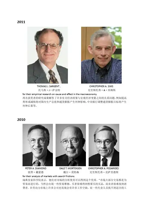
2011THOMAS J. SARGENT , CHRISTOPHER A. SIMS托马斯·J·萨金特克里斯托弗·A·西姆斯for their empirical research on cause and effect in the macroeconomy.两名获奖者的研究成果解答了许多有关经济政策与宏观经济变量之间的关系问题，例如提高利率或减税将对国内生产总值和通货膨胀产生何种影响，中央银行调整通货膨胀目标将产生何种后果等。

2010PETER A. DIAMOND DALE T. MORTENSEN CHRISTOPHER A. PISSARIDES彼得·戴蒙德戴尔·莫特森克里斯托弗·皮萨里德斯for their analysis of markets with search frictions.瑞典皇家科学院表示，他们对市场的分析使其可以得到这个奖项。

“市场大部分交易都是为贸易而进行的，当然会出现一些贸易摩擦，买者很难得到想要买的买品，而卖者很难找到消费者。

在劳动力市场上许多公司也发现会有许多工作空缺，而一些失业人员找不到适合的工作岗位。

”彼特-戴蒙德等人所开发的理论是解释了市场上这种冲突，他们的理论是基于微观经济学理论的，也就是市场合理产出，他们的工作也就是意味着雇佣工人要更加合理，在招聘人员和需求工作应该提供合理的机制。

2009ELINOR OSTROM OLIVER E. WILLIAMSON埃莉诺·奥斯特罗姆奥利弗·E·威廉姆森for her analysis of economic governance, especially the commons表彰她对经济治理的分析，尤其是对普通人经济治理活动的研究for his analysis of economic governance, especially the boundaries of the firm表彰他对经济治理的分析，特别是对公司的经济治理边界的分析2008PAUL KRUGMAN保罗·克鲁格曼for his analysis of trade patterns and location of economic activity.在贸易模式上所做的分析工作和对经济活动的定位2007LEONID HURWICZ ERIC S. MASKIN ROGER B. MYERSON莱昂尼德·赫维奇埃里克·马斯金罗杰·迈尔森for having laid the foundations of mechanism design theory.为机制设计理论（Mechanism Design Theory）奠定了基础2006EDMUND S. PHELPS埃德蒙德·菲尔普斯for his analysis of intertemporal tradeoffs in macroeconomic policy.加深人们对于通货膨胀和失业预期关系的理解方面所做的贡献2005ROBERT J. AUMANN THOMAS C. SCHELLING罗伯特·约翰·奥曼托马斯·克罗姆比·谢林for having enhanced our understanding of conflict and cooperation through game-theory analysis.通过博弈论分析促进了对冲突与合作的理解2004FINN E. KYDLAND EDWARD C. PRESCOTT芬恩·基德兰德爱德华·普雷斯科特for their contributions to dynamic macroeconomics: the time consistency of economic policy and the driving forces behind business cycles通过对宏观经济政策运用中“时间连贯性难题”的分析研究，为经济政策特别是货币政策的实际有效运用提供了思路；二是在对商业周期的研究中，通过对引起商业周期波动的各种因素和各因素间相互关系的分析，使人们对于这一现象的认识更加深入2003ROBERT F. ENGLE CLIVE W. J. GRANGER罗伯特·恩格尔克莱夫·格兰杰for methods of analyzing economic time series with time-varying volatility (ARCH)表彰罗伯特·恩格尔使用“随着时间变化的易变性”新方法分析经济时间序列，从而给经济学研究和经济发展带来巨大影响for methods of analyzing economic time series with common trends (cointegration)表彰克莱夫·格兰杰使用“共同趋势”新方法分析经济时间序列，从而给经济学研究和经济发展带来巨大影响2002DANIEL KAHNEMAN VERNON L. SMITH,丹尼尔·卡纳曼弗农·史密斯for having integrated insights from psychological research into economic science, especially concerning human judgment and decision-making under uncertainty表彰丹尼尔·卡纳曼用认知心理学分析方法研究人类的判断和决策行为的领域for having established laboratory experiments as a tool in empirical economic analysis, especially in the study of alternative market mechanisms表彰弗农·史密斯通过实验室实验来测试或检验根据经济学理论作出预测的未知或不确定性领域2001GEORGE A. AKERLOF A. MICHAEL SPENCE JOSEPH E. STIGLITZ乔治·阿克尔洛夫迈克尔·斯宾塞约瑟夫·斯蒂格利茨for their analyses of markets with asymmetric information.为不对称信息市场的一般理论奠定了基石2000JAMES J. HECKMAN DANIEL L. MCFADDEN詹姆斯·赫克曼丹尼尔·麦克法登for his development of theory and methods for analyzing selective samples表彰詹姆斯·赫克曼对分析选择性抽样的原理和方法所做出的发展和贡献for his development of theory and methods for analyzing discrete choice.表彰丹尼尔·麦克法登对分析离散选择的原理和方法所做出的发展和贡献1999ROBERT A. MUNDELL罗伯特·蒙代尔for his analysis of monetary and fiscal policy under different exchange rate regimes and his analysis of optimum currency areas.表彰他对不同汇率体制下货币与财政政策以及最适宜的货币流通区域所做的分析1998AMATYA SEN阿马蒂亚·森for his contributions to welfare economics.对福利经济学几个重大问题做出了贡献，包括社会选择理论、对福利和贫穷标准的定义、对匮乏的研究等1997ROBERT C. MERTON MYRON S. SCHOLES罗伯特·默顿迈伦·斯科尔斯for a new method to determine the value of derivatives.前者对布莱克－斯科尔斯公式所依赖的假设条件做了进一步减弱，在许多方面对其做了推广。

Network impacts of a road capacity reduction:Empirical analysisand model predictionsDavid Watling a ,⇑,David Milne a ,Stephen Clark baInstitute for Transport Studies,University of Leeds,Woodhouse Lane,Leeds LS29JT,UK b Leeds City Council,Leonardo Building,2Rossington Street,Leeds LS28HD,UKa r t i c l e i n f o Article history:Received 24May 2010Received in revised form 15July 2011Accepted 7September 2011Keywords:Traffic assignment Network models Equilibrium Route choice Day-to-day variabilitya b s t r a c tIn spite of their widespread use in policy design and evaluation,relatively little evidencehas been reported on how well traffic equilibrium models predict real network impacts.Here we present what we believe to be the first paper that together analyses the explicitimpacts on observed route choice of an actual network intervention and compares thiswith the before-and-after predictions of a network equilibrium model.The analysis isbased on the findings of an empirical study of the travel time and route choice impactsof a road capacity reduction.Time-stamped,partial licence plates were recorded across aseries of locations,over a period of days both with and without the capacity reduction,and the data were ‘matched’between locations using special-purpose statistical methods.Hypothesis tests were used to identify statistically significant changes in travel times androute choice,between the periods of days with and without the capacity reduction.A trafficnetwork equilibrium model was then independently applied to the same scenarios,and itspredictions compared with the empirical findings.From a comparison of route choice pat-terns,a particularly influential spatial effect was revealed of the parameter specifying therelative values of distance and travel time assumed in the generalised cost equations.When this parameter was ‘fitted’to the data without the capacity reduction,the networkmodel broadly predicted the route choice impacts of the capacity reduction,but with othervalues it was seen to perform poorly.The paper concludes by discussing the wider practicaland research implications of the study’s findings.Ó2011Elsevier Ltd.All rights reserved.1.IntroductionIt is well known that altering the localised characteristics of a road network,such as a planned change in road capacity,will tend to have both direct and indirect effects.The direct effects are imparted on the road itself,in terms of how it can deal with a given demand flow entering the link,with an impact on travel times to traverse the link at a given demand flow level.The indirect effects arise due to drivers changing their travel decisions,such as choice of route,in response to the altered travel times.There are many practical circumstances in which it is desirable to forecast these direct and indirect impacts in the context of a systematic change in road capacity.For example,in the case of proposed road widening or junction improvements,there is typically a need to justify econom-ically the required investment in terms of the benefits that will likely accrue.There are also several examples in which it is relevant to examine the impacts of road capacity reduction .For example,if one proposes to reallocate road space between alternative modes,such as increased bus and cycle lane provision or a pedestrianisation scheme,then typically a range of alternative designs exist which may differ in their ability to accommodate efficiently the new traffic and routing patterns.0965-8564/$-see front matter Ó2011Elsevier Ltd.All rights reserved.doi:10.1016/j.tra.2011.09.010⇑Corresponding author.Tel.:+441133436612;fax:+441133435334.E-mail address:d.p.watling@ (D.Watling).168 D.Watling et al./Transportation Research Part A46(2012)167–189Through mathematical modelling,the alternative designs may be tested in a simulated environment and the most efficient selected for implementation.Even after a particular design is selected,mathematical models may be used to adjust signal timings to optimise the use of the transport system.Road capacity may also be affected periodically by maintenance to essential services(e.g.water,electricity)or to the road itself,and often this can lead to restricted access over a period of days and weeks.In such cases,planning authorities may use modelling to devise suitable diversionary advice for drivers,and to plan any temporary changes to traffic signals or priorities.Berdica(2002)and Taylor et al.(2006)suggest more of a pro-ac-tive approach,proposing that models should be used to test networks for potential vulnerability,before any reduction mate-rialises,identifying links which if reduced in capacity over an extended period1would have a substantial impact on system performance.There are therefore practical requirements for a suitable network model of travel time and route choice impacts of capac-ity changes.The dominant method that has emerged for this purpose over the last decades is clearly the network equilibrium approach,as proposed by Beckmann et al.(1956)and developed in several directions since.The basis of using this approach is the proposition of what are believed to be‘rational’models of behaviour and other system components(e.g.link perfor-mance functions),with site-specific data used to tailor such models to particular case studies.Cross-sectional forecasts of network performance at specific road capacity states may then be made,such that at the time of any‘snapshot’forecast, drivers’route choices are in some kind of individually-optimum state.In this state,drivers cannot improve their route selec-tion by a unilateral change of route,at the snapshot travel time levels.The accepted practice is to‘validate’such models on a case-by-case basis,by ensuring that the model—when supplied with a particular set of parameters,input network data and input origin–destination demand data—reproduces current mea-sured mean link trafficflows and mean journey times,on a sample of links,to some degree of accuracy(see for example,the practical guidelines in TMIP(1997)and Highways Agency(2002)).This kind of aggregate level,cross-sectional validation to existing conditions persists across a range of network modelling paradigms,ranging from static and dynamic equilibrium (Florian and Nguyen,1976;Leonard and Tough,1979;Stephenson and Teply,1984;Matzoros et al.,1987;Janson et al., 1986;Janson,1991)to micro-simulation approaches(Laird et al.,1999;Ben-Akiva et al.,2000;Keenan,2005).While such an approach is plausible,it leaves many questions unanswered,and we would particularly highlight two: 1.The process of calibration and validation of a network equilibrium model may typically occur in a cycle.That is to say,having initially calibrated a model using the base data sources,if the subsequent validation reveals substantial discrep-ancies in some part of the network,it is then natural to adjust the model parameters(including perhaps even the OD matrix elements)until the model outputs better reflect the validation data.2In this process,then,we allow the adjustment of potentially a large number of network parameters and input data in order to replicate the validation data,yet these data themselves are highly aggregate,existing only at the link level.To be clear here,we are talking about a level of coarseness even greater than that in aggregate choice models,since we cannot even infer from link-level data the aggregate shares on alternative routes or OD movements.The question that arises is then:how many different combinations of parameters and input data values might lead to a similar link-level validation,and even if we knew the answer to this question,how might we choose between these alternative combinations?In practice,this issue is typically neglected,meaning that the‘valida-tion’is a rather weak test of the model.2.Since the data are cross-sectional in time(i.e.the aim is to reproduce current base conditions in equilibrium),then in spiteof the large efforts required in data collection,no empirical evidence is routinely collected regarding the model’s main purpose,namely its ability to predict changes in behaviour and network performance under changes to the network/ demand.This issue is exacerbated by the aggregation concerns in point1:the‘ambiguity’in choosing appropriate param-eter values to satisfy the aggregate,link-level,base validation strengthens the need to independently verify that,with the selected parameter values,the model responds reliably to changes.Although such problems–offitting equilibrium models to cross-sectional data–have long been recognised by practitioners and academics(see,e.g.,Goodwin,1998), the approach described above remains the state-of-practice.Having identified these two problems,how might we go about addressing them?One approach to thefirst problem would be to return to the underlying formulation of the network model,and instead require a model definition that permits analysis by statistical inference techniques(see for example,Nakayama et al.,2009).In this way,we may potentially exploit more information in the variability of the link-level data,with well-defined notions(such as maximum likelihood)allowing a systematic basis for selection between alternative parameter value combinations.However,this approach is still using rather limited data and it is natural not just to question the model but also the data that we use to calibrate and validate it.Yet this is not altogether straightforward to resolve.As Mahmassani and Jou(2000) remarked:‘A major difficulty...is obtaining observations of actual trip-maker behaviour,at the desired level of richness, simultaneously with measurements of prevailing conditions’.For this reason,several authors have turned to simulated gaming environments and/or stated preference techniques to elicit information on drivers’route choice behaviour(e.g. 1Clearly,more sporadic and less predictable reductions in capacity may also occur,such as in the case of breakdowns and accidents,and environmental factors such as severe weather,floods or landslides(see for example,Iida,1999),but the responses to such cases are outside the scope of the present paper. 2Some authors have suggested more systematic,bi-level type optimization processes for thisfitting process(e.g.Xu et al.,2004),but this has no material effect on the essential points above.D.Watling et al./Transportation Research Part A46(2012)167–189169 Mahmassani and Herman,1990;Iida et al.,1992;Khattak et al.,1993;Vaughn et al.,1995;Wardman et al.,1997;Jou,2001; Chen et al.,2001).This provides potentially rich information for calibrating complex behavioural models,but has the obvious limitation that it is based on imagined rather than real route choice situations.Aside from its common focus on hypothetical decision situations,this latter body of work also signifies a subtle change of emphasis in the treatment of the overall network calibration problem.Rather than viewing the network equilibrium calibra-tion process as a whole,the focus is on particular components of the model;in the cases above,the focus is on that compo-nent concerned with how drivers make route decisions.If we are prepared to make such a component-wise analysis,then certainly there exists abundant empirical evidence in the literature,with a history across a number of decades of research into issues such as the factors affecting drivers’route choice(e.g.Wachs,1967;Huchingson et al.,1977;Abu-Eisheh and Mannering,1987;Duffell and Kalombaris,1988;Antonisse et al.,1989;Bekhor et al.,2002;Liu et al.,2004),the nature of travel time variability(e.g.Smeed and Jeffcoate,1971;Montgomery and May,1987;May et al.,1989;McLeod et al., 1993),and the factors affecting trafficflow variability(Bonsall et al.,1984;Huff and Hanson,1986;Ribeiro,1994;Rakha and Van Aerde,1995;Fox et al.,1998).While these works provide useful evidence for the network equilibrium calibration problem,they do not provide a frame-work in which we can judge the overall‘fit’of a particular network model in the light of uncertainty,ambient variation and systematic changes in network attributes,be they related to the OD demand,the route choice process,travel times or the network data.Moreover,such data does nothing to address the second point made above,namely the question of how to validate the model forecasts under systematic changes to its inputs.The studies of Mannering et al.(1994)and Emmerink et al.(1996)are distinctive in this context in that they address some of the empirical concerns expressed in the context of travel information impacts,but their work stops at the stage of the empirical analysis,without a link being made to net-work prediction models.The focus of the present paper therefore is both to present thefindings of an empirical study and to link this empirical evidence to network forecasting models.More recently,Zhu et al.(2010)analysed several sources of data for evidence of the traffic and behavioural impacts of the I-35W bridge collapse in Minneapolis.Most pertinent to the present paper is their location-specific analysis of linkflows at 24locations;by computing the root mean square difference inflows between successive weeks,and comparing the trend for 2006with that for2007(the latter with the bridge collapse),they observed an apparent transient impact of the bridge col-lapse.They also showed there was no statistically-significant evidence of a difference in the pattern offlows in the period September–November2007(a period starting6weeks after the bridge collapse),when compared with the corresponding period in2006.They suggested that this was indicative of the length of a‘re-equilibration process’in a conceptual sense, though did not explicitly compare their empiricalfindings with those of a network equilibrium model.The structure of the remainder of the paper is as follows.In Section2we describe the process of selecting the real-life problem to analyse,together with the details and rationale behind the survey design.Following this,Section3describes the statistical techniques used to extract information on travel times and routing patterns from the survey data.Statistical inference is then considered in Section4,with the aim of detecting statistically significant explanatory factors.In Section5 comparisons are made between the observed network data and those predicted by a network equilibrium model.Finally,in Section6the conclusions of the study are highlighted,and recommendations made for both practice and future research.2.Experimental designThe ultimate objective of the study was to compare actual data with the output of a traffic network equilibrium model, specifically in terms of how well the equilibrium model was able to correctly forecast the impact of a systematic change ap-plied to the network.While a wealth of surveillance data on linkflows and travel times is routinely collected by many local and national agencies,we did not believe that such data would be sufficiently informative for our purposes.The reason is that while such data can often be disaggregated down to small time step resolutions,the data remains aggregate in terms of what it informs about driver response,since it does not provide the opportunity to explicitly trace vehicles(even in aggre-gate form)across more than one location.This has the effect that observed differences in linkflows might be attributed to many potential causes:it is especially difficult to separate out,say,ambient daily variation in the trip demand matrix from systematic changes in route choice,since both may give rise to similar impacts on observed linkflow patterns across re-corded sites.While methods do exist for reconstructing OD and network route patterns from observed link data(e.g.Yang et al.,1994),these are typically based on the premise of a valid network equilibrium model:in this case then,the data would not be able to give independent information on the validity of the network equilibrium approach.For these reasons it was decided to design and implement a purpose-built survey.However,it would not be efficient to extensively monitor a network in order to wait for something to happen,and therefore we required advance notification of some planned intervention.For this reason we chose to study the impact of urban maintenance work affecting the roads,which UK local government authorities organise on an annual basis as part of their‘Local Transport Plan’.The city council of York,a historic city in the north of England,agreed to inform us of their plans and to assist in the subsequent data collection exercise.Based on the interventions planned by York CC,the list of candidate studies was narrowed by considering factors such as its propensity to induce significant re-routing and its impact on the peak periods.Effectively the motivation here was to identify interventions that were likely to have a large impact on delays,since route choice impacts would then likely be more significant and more easily distinguished from ambient variability.This was notably at odds with the objectives of York CC,170 D.Watling et al./Transportation Research Part A46(2012)167–189in that they wished to minimise disruption,and so where possible York CC planned interventions to take place at times of day and of the year where impacts were minimised;therefore our own requirement greatly reduced the candidate set of studies to monitor.A further consideration in study selection was its timing in the year for scheduling before/after surveys so to avoid confounding effects of known significant‘seasonal’demand changes,e.g.the impact of the change between school semesters and holidays.A further consideration was York’s role as a major tourist attraction,which is also known to have a seasonal trend.However,the impact on car traffic is relatively small due to the strong promotion of public trans-port and restrictions on car travel and parking in the historic centre.We felt that we further mitigated such impacts by sub-sequently choosing to survey in the morning peak,at a time before most tourist attractions are open.Aside from the question of which intervention to survey was the issue of what data to collect.Within the resources of the project,we considered several options.We rejected stated preference survey methods as,although they provide a link to personal/socio-economic drivers,we wanted to compare actual behaviour with a network model;if the stated preference data conflicted with the network model,it would not be clear which we should question most.For revealed preference data, options considered included(i)self-completion diaries(Mahmassani and Jou,2000),(ii)automatic tracking through GPS(Jan et al.,2000;Quiroga et al.,2000;Taylor et al.,2000),and(iii)licence plate surveys(Schaefer,1988).Regarding self-comple-tion surveys,from our own interview experiments with self-completion questionnaires it was evident that travellersfind it relatively difficult to recall and describe complex choice options such as a route through an urban network,giving the po-tential for significant errors to be introduced.The automatic tracking option was believed to be the most attractive in this respect,in its potential to accurately map a given individual’s journey,but the negative side would be the potential sample size,as we would need to purchase/hire and distribute the devices;even with a large budget,it is not straightforward to identify in advance the target users,nor to guarantee their cooperation.Licence plate surveys,it was believed,offered the potential for compromise between sample size and data resolution: while we could not track routes to the same resolution as GPS,by judicious location of surveyors we had the opportunity to track vehicles across more than one location,thus providing route-like information.With time-stamped licence plates, the matched data would also provide journey time information.The negative side of this approach is the well-known poten-tial for significant recording errors if large sample rates are required.Our aim was to avoid this by recording only partial licence plates,and employing statistical methods to remove the impact of‘spurious matches’,i.e.where two different vehi-cles with the same partial licence plate occur at different locations.Moreover,extensive simulation experiments(Watling,1994)had previously shown that these latter statistical methods were effective in recovering the underlying movements and travel times,even if only a relatively small part of the licence plate were recorded,in spite of giving a large potential for spurious matching.We believed that such an approach reduced the opportunity for recorder error to such a level to suggest that a100%sample rate of vehicles passing may be feasible.This was tested in a pilot study conducted by the project team,with dictaphones used to record a100%sample of time-stamped, partial licence plates.Independent,duplicate observers were employed at the same location to compare error rates;the same study was also conducted with full licence plates.The study indicated that100%surveys with dictaphones would be feasible in moderate trafficflow,but only if partial licence plate data were used in order to control observation errors; for higherflow rates or to obtain full number plate data,video surveys should be considered.Other important practical les-sons learned from the pilot included the need for clarity in terms of vehicle types to survey(e.g.whether to include motor-cycles and taxis),and of the phonetic alphabet used by surveyors to avoid transcription ambiguities.Based on the twin considerations above of planned interventions and survey approach,several candidate studies were identified.For a candidate study,detailed design issues involved identifying:likely affected movements and alternative routes(using local knowledge of York CC,together with an existing network model of the city),in order to determine the number and location of survey sites;feasible viewpoints,based on site visits;the timing of surveys,e.g.visibility issues in the dark,winter evening peak period;the peak duration from automatic trafficflow data;and specific survey days,in view of public/school holidays.Our budget led us to survey the majority of licence plate sites manually(partial plates by audio-tape or,in lowflows,pen and paper),with video surveys limited to a small number of high-flow sites.From this combination of techniques,100%sampling rate was feasible at each site.Surveys took place in the morning peak due both to visibility considerations and to minimise conflicts with tourist/special event traffic.From automatic traffic count data it was decided to survey the period7:45–9:15as the main morning peak period.This design process led to the identification of two studies:2.1.Lendal Bridge study(Fig.1)Lendal Bridge,a critical part of York’s inner ring road,was scheduled to be closed for maintenance from September2000 for a duration of several weeks.To avoid school holidays,the‘before’surveys were scheduled for June and early September.It was decided to focus on investigating a significant southwest-to-northeast movement of traffic,the river providing a natural barrier which suggested surveying the six river crossing points(C,J,H,K,L,M in Fig.1).In total,13locations were identified for survey,in an attempt to capture traffic on both sides of the river as well as a crossing.2.2.Fishergate study(Fig.2)The partial closure(capacity reduction)of the street known as Fishergate,again part of York’s inner ring road,was scheduled for July2001to allow repairs to a collapsed sewer.Survey locations were chosen in order to intercept clockwiseFig.1.Intervention and survey locations for Lendal Bridge study.around the inner ring road,this being the direction of the partial closure.A particular aim wasFulford Road(site E in Fig.2),the main radial affected,with F and K monitoring local diversion I,J to capture wider-area diversion.studies,the plan was to survey the selected locations in the morning peak over a period of approximately covering the three periods before,during and after the intervention,with the days selected so holidays or special events.Fig.2.Intervention and survey locations for Fishergate study.In the Lendal Bridge study,while the‘before’surveys proceeded as planned,the bridge’s actualfirst day of closure on Sep-tember11th2000also marked the beginning of the UK fuel protests(BBC,2000a;Lyons and Chaterjee,2002).Trafficflows were considerably affected by the scarcity of fuel,with congestion extremely low in thefirst week of closure,to the extent that any changes could not be attributed to the bridge closure;neither had our design anticipated how to survey the impacts of the fuel shortages.We thus re-arranged our surveys to monitor more closely the planned re-opening of the bridge.Unfor-tunately these surveys were hampered by a second unanticipated event,namely the wettest autumn in the UK for270years and the highest level offlooding in York since records began(BBC,2000b).Theflooding closed much of the centre of York to road traffic,including our study area,as the roads were impassable,and therefore we abandoned the planned‘after’surveys. As a result of these events,the useable data we had(not affected by the fuel protests orflooding)consisted offive‘before’days and one‘during’day.In the Fishergate study,fortunately no extreme events occurred,allowing six‘before’and seven‘during’days to be sur-veyed,together with one additional day in the‘during’period when the works were temporarily removed.However,the works over-ran into the long summer school holidays,when it is well-known that there is a substantial seasonal effect of much lowerflows and congestion levels.We did not believe it possible to meaningfully isolate the impact of the link fully re-opening while controlling for such an effect,and so our plans for‘after re-opening’surveys were abandoned.3.Estimation of vehicle movements and travel timesThe data resulting from the surveys described in Section2is in the form of(for each day and each study)a set of time-stamped,partial licence plates,observed at a number of locations across the network.Since the data include only partial plates,they cannot simply be matched across observation points to yield reliable estimates of vehicle movements,since there is ambiguity in whether the same partial plate observed at different locations was truly caused by the same vehicle. Indeed,since the observed system is‘open’—in the sense that not all points of entry,exit,generation and attraction are mon-itored—the question is not just which of several potential matches to accept,but also whether there is any match at all.That is to say,an apparent match between data at two observation points could be caused by two separate vehicles that passed no other observation point.Thefirst stage of analysis therefore applied a series of specially-designed statistical techniques to reconstruct the vehicle movements and point-to-point travel time distributions from the observed data,allowing for all such ambiguities in the data.Although the detailed derivations of each method are not given here,since they may be found in the references provided,it is necessary to understand some of the characteristics of each method in order to interpret the results subsequently provided.Furthermore,since some of the basic techniques required modification relative to the published descriptions,then in order to explain these adaptations it is necessary to understand some of the theoretical basis.3.1.Graphical method for estimating point-to-point travel time distributionsThe preliminary technique applied to each data set was the graphical method described in Watling and Maher(1988).This method is derived for analysing partial registration plate data for unidirectional movement between a pair of observation stations(referred to as an‘origin’and a‘destination’).Thus in the data study here,it must be independently applied to given pairs of observation stations,without regard for the interdependencies between observation station pairs.On the other hand, it makes no assumption that the system is‘closed’;there may be vehicles that pass the origin that do not pass the destina-tion,and vice versa.While limited in considering only two-point surveys,the attraction of the graphical technique is that it is a non-parametric method,with no assumptions made about the arrival time distributions at the observation points(they may be non-uniform in particular),and no assumptions made about the journey time probability density.It is therefore very suitable as afirst means of investigative analysis for such data.The method begins by forming all pairs of possible matches in the data,of which some will be genuine matches(the pair of observations were due to a single vehicle)and the remainder spurious matches.Thus, for example,if there are three origin observations and two destination observations of a particular partial registration num-ber,then six possible matches may be formed,of which clearly no more than two can be genuine(and possibly only one or zero are genuine).A scatter plot may then be drawn for each possible match of the observation time at the origin versus that at the destination.The characteristic pattern of such a plot is as that shown in Fig.4a,with a dense‘line’of points(which will primarily be the genuine matches)superimposed upon a scatter of points over the whole region(which will primarily be the spurious matches).If we were to assume uniform arrival rates at the observation stations,then the spurious matches would be uniformly distributed over this plot;however,we shall avoid making such a restrictive assumption.The method begins by making a coarse estimate of the total number of genuine matches across the whole of this plot.As part of this analysis we then assume knowledge of,for any randomly selected vehicle,the probabilities:h k¼Prðvehicle is of the k th type of partial registration plateÞðk¼1;2;...;mÞwhereX m k¼1h k¼1172 D.Watling et al./Transportation Research Part A46(2012)167–189。