北大光华宏观讲义notes2
- 格式:pdf
- 大小:1.34 MB
- 文档页数:44

北大讲义国际金融学专题开放经济调价下的宏观调控Standardization of sany group #QS8QHH-HHGX8Q8-GNHHJ8-HHMHGN#(2)开放条件下的政策目标之间关系——米德冲突经济学家詹姆斯·米德于1951年在《国际收支》中最早提出了下的内外均衡冲突问题,称为“米德冲突”:在固定不变时,政府只能主要运用影响的政策来调节内外均衡,如果单一的使用某种政策,在运行的特定区间往往会出现内外均衡难以兼顾的情形。
在米德的分析中,的冲突一般是指在下,高失业率、国际收支逆差或高通货膨胀、国际收支顺差这两种特定的内外经济状况组合。
内部不平衡外部不平衡财政政策调节1 高失业率国际收支逆差冲突2 高通货膨胀率国际收支顺差冲突情形1:为了降低失业率而采取扩张性财政政策,将带来国际收支逆差的扩大;若通过宽松的货币政策减少失业,利率下降至资本项目逆差增加,国内物价上升至经常项目逆差增加。
情形2:为了降低通胀率而采取紧缩性财政政策,将带来国际收支顺差的扩大;若通过紧缩的货币政策降低通胀率,利率上升至资本项目顺差增加,国内价格下降至经常项目顺差增加。
——在情形1、情形2下,单一使用财政政策或货币政策都难以兼顾内部平衡与外部平衡目标。
(3)开放条件下宏观调控的基本思路丁伯根原则丁伯根认为一国政府要实现一个经济目标需要至少一个有效的政策工具,要实现N个独立的经济目标,至少需要使用N个独立有效的政策工具。
显然在丁伯根准则下,在固定汇率制度下,单一的财政政策(或货币政策)无法协调内部平衡与外部平衡两个独立的目标。
简·丁伯根(1903—1994),荷兰海牙人,计量经济学之父,1969年与拉格纳·弗里希共同获得首届诺贝尔经济学奖。
蒙代尔原则如果每一个工具都能够被合理的指派给某一个目标,并且在该目标偏离其最佳水平时按照规则进行调整,那么在分散决策的情况下,仍有可能实现最佳调控目标。
北大光华管理学院考研辅导班课程讲义精讲各位考研的同学们,大家好!我是才思的一名学员,现在已经顺利的考上北大管理学院,今天和大家分享一下这个专业的笔记,方便大家准备考研,希望给大家一定的帮助。
170.证券市场的“三公”原则建立和维护证券市场的公开、公平、公正的“三公”原则,是保护投资盲合法利益不受侵犯的基本原则,也是保护投资者利益的基础。
“三公”原则的具体内容包括:(1)公开原则,又称信息公开原则。
公开原则通常包括两个方面,即证券信息的初期披露和持续披露。
(2)公平原则。
证券市场的公平原则,要求证券发行、交易活动中的所有参与者都有平等的法律地位,各自的合法权益能够得到公平的保护。
(3)公正原则。
公正原则是针对证券监管机构的监管行为而言的,它要求证券监督管理部门在公开、公平原则基础上,对一切被监管对象给以公正待遇。
171.内幕交易内幕交易主要包括下列行为:①内幕人员利用内幕信息买卖证券,或者根据内幕信息建议他人买卖证券的行为;②内幕人员向他人泄漏内幕信息,使他人利用该信息获利的行为;③非内幕人员通过不正当的手段或者其他途径获得内幕信息,并根据该内幕信息买卖证券,或者建议他人买卖证券的行为。
这里的内幕人员,是指上市公司的董事会、监事会人员及其他高级管理人员,证券市场的主管机关和证券中介机构的工作人员,以及为该上市公司服务的律师、会计师等能够接触或者获得内幕信息的人员。
172.关联交易关联交易就是企业关联方之间的交易。
根据财政部1997年5月22日颁布的《企业会计准则——关联方关系及其交易的披露》的规定、在企业财务和经营决策中。
如果一方有能力直接或间接控制,共同拧制另一方或对另一方施加重大影响,则视其为关联方;如果两方或多方受同一方控制,也将具视为关联方。
凡以上关联方之间发生转移资源或义务的事项,不论是否收取价款,均破视为关联交易。
173、过度包装股份公司借上中的机会进行适当的包装,有利于塑造更好的企业形象,增强对投资者的吸引力。

课程说明1.本课程为金融学专业硕士生的必修课程,系统地讲授课程说明1.授课方式:讲授课程说明1.评估方法课程说明1.授课教师:唐国正教学内容1.什么是金融工程?什么是金融工程?定义1.包括设计、开发和实施具有创新意义的金融工具和金什么是金融工程?创新1.创新的三个层次什么是金融工程?金融工程产品作为金融创新活动的结果,金融工程产品可能是教学内容1.什么是金融工程?金融创新的动机税法与监管的变化1.Merton Miller认为:金融创新的动机减少金融约束1.Silber认为金融创新的过程实质上是公司试图放松面金融创新的社会价值R. C. Merton认为金融创新可以从三个方面提升经济公司(RJR金融创新的社会价值零和对策?1.许多经济学家认为,从全社会的角度来看,以绕开监教学内容1.什么是金融工程?金融工程的创新标准1.一种金融工具或者金融策略成为一项金融创新的条件金融工程的创新标准1.如果用Van Horne的标准来衡量,那么一些过去被认金融工程的创新标准债权-股权互换的税收套利1.A公司:金融工程的创新标准债权-股权互换的税收套利1.这笔交易对A公司来说是有意义的教学内容1.什么是金融工程?推动金融工程发展的因素在综合了Miller、Silber与Van Horne的研究成果教学内容1.什么是金融工程?应用领域综述1.开展金融工程活动的主体应用领域融资1.在融资方面,一种类型的金融工程活动是:在各种约应用领域融资4.另一种类型的金融工程活动与公司并购有关,在并购应用领域投资与现金管理1.在投资方面,金融工程师开发出了各种各样的中长期应用领域管理发行人的风险1.在风险管理领域,金融工程发挥着重要作用应用领域管理投资者的风险1.挑战性q90年代市场上出现的与股票指数挂钩的债券应用领域风险管理管理投资者的风险与管理发行人的风险迥然不同应用领域套利1.开发交易策略来利用不同地点、不同时间、不同工具教学内容1.什么是金融工程?应用领域非金融类公司1.金融工程在公司层面有着非常重要的应用应用领域非金融类公司1.对公司来说,金融工程可以用来应用领域非金融类公司安然公司(Enron) 应用领域非金融类公司1.1993年,为了便于供应商与最终消费者管理价格风教学内容1.什么是金融工程?理论基础1.作为一门应用学科,金融工程的理论基础主要来自于基本工具1.金融工程的工具可以分成两部分,一部分是基本的金来,用以实现某一特定的目标其它理论、工具1.除了应用上述理论与工具以外,金融工程活动常常还。

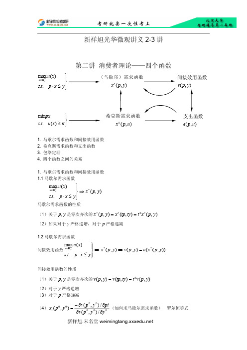
北京大学宏观经济学考研笔记讲义萨克斯宏观经济学第一章导论宏观经济学的定义:宏观经济学是一门研究经济总体行为的经济学科。
它研究由各经济主体的行为所决定的经济总量(产出、消费、储蓄、投资、贸易余额、财政赤字)之间的关系,名义变量(货币供给、物价水平、汇率)与实际变量之间的关系,以及在减少经济波动、保持物价水平和实现稳定增长方面宏观经济政策的作用。
宏观经济学研究的3个步骤:1、宏观经济学家试图在理论水平上理解单个企业和家庭的决策过程。
2、试图加总经济中个别家庭和企业的所有决策,来解释经济的整体行为。
3、通过收集并分析实际宏观经济数据,为理论提供经验内容。
四个关键问题:1、商业周期2、失业率3、通货膨胀率4、贸易余额宏观经济学研究的目的:1、充分就业2、物价稳定3、国际收支平衡4、经济增长凯恩斯《就业、利息和货币通论》的中心论点:市场并不能平滑地自我调节,不能保证常规的低水平失业和高水平生产;政府可以实施稳定政策以防止或抑制经济衰退。
凯恩斯革命:1、由于乐观主义和悲观主义之间的摇摆,会影响商业投资总水平,从而造成经济较大的波动。
2、像大萧条这样深重的经济衰退一旦出现,单靠市场力量是不可能迅速消除的。
3、只有宏观经济政策,特别是政府支出和税收以及货币政策进行重大调整,才能阻止经济衰退、保持经济稳定。
反凯恩斯革命:70年代,经济前景暗淡,很多国家经历了滞胀。
凯恩斯学派的政策建议对这种特定的经济困境似乎无可奈何。
许多经济学家和非经济学家认识到,稳定政策实际上正是在此发生不稳定的主要原因。
人们指责积极的政府政策本身是滞胀的原因之一。
货币主义:以弗里德曼为首的货币主义者认为市场经济是自我调节的,如果不加干预,经济会倾向自行恢复充分就业;其次,他们认为积极的宏观经济政策只会造成问题,而不会解决问题。
《美国货币史》指出,经济波动在很大程度上是货币供应发生变化的结果,稳定的货币供应而非变化的货币供应,才是稳定宏观经济的真正关键。

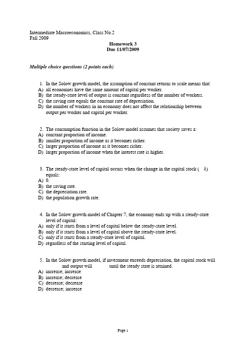
Intermediate Macroeconomics, Class No.2Fall 2009Homework 3Due 11/07/2009Multiple choice questions (2 points each)1. In the Solow growth model, the assumption of constant returns to scale means that:A) all economies have the same amount of capital per worker.B) the steady-state level of output is constant regardless of the number of workers.C) the saving rate equals the constant rate of depreciation.D) the number of workers in an economy does not affect the relationship betweenoutput per worker and capital per worker.2. The consumption function in the Solow model assumes that society saves a:A) constant proportion of income.B) smaller proportion of income as it becomes richer.C) larger proportion of income as it becomes richer.D) larger proportion of income when the interest rate is higher.3. The steady-state level of capital occurs when the change in the capital stock ( k)equals:A) 0.B) the saving rate.C) the depreciation rate.D) the population growth rate.4. In the Solow growth model of Chapter 7, the economy ends up with a steady-statelevel of capital:A) only if it starts from a level of capital below the steady-state level.B) only if it starts from a level of capital above the steady-state level.C) only if it starts from a steady-state level of capital.D) regardless of the starting level of capital.5. In the Solow growth model, if investment exceeds depreciation, the capital stock will______ and output will ______ until the steady state is attained.A) increase; increaseB) increase; decreaseC) decrease; decreaseD) decrease; increase6. If the per-worker production function is given by y = k1/2, the saving rate (s) is 0.2,and the depreciation rate is 0.1, then the steady-state ratio of capital to labor is:A) 1.B) 2.C) 4.D) 9.7. If a war destroys a large portion of a country's capital stock but the saving rate isunchanged, the Solow model predicts output will grow and that the new steady state will approach:A) a higher output level than before.B) the same output level as before.C) a lower output level than before.D) the Golden Rule output level.8. If the national saving rate increases, the:A) economy will grow at a faster rate forever.B) capital-labor ratio will increase forever.C) economy will grow at a faster rate until a new, higher, steady-state capital-labor ratiois reached.D) capital-labor ratio will eventually decline.9. A higher saving rate leads to a:A) higher rate of economic growth in both the short run and the long run.B) higher rate of economic growth only in the long run.C) higher rate of economic growth in the short run but a decline in the long run.D) large capital stock and a high level of output in the long run.10. The Golden Rule level of the steady-state capital stock:A) will be reached automatically if the saving rate remains constant over a long periodof time.B) will be reached automatically if each person saves enough to provide for his or herretirement.C) implies a choice of a particular saving rate.D) should be avoided by an enlightened government.11. If y = k1/2, there is no population growth or technological progress, 5 percent ofcapital depreciates each year, and a country saves 20 percent of output each year, then the steady-state level of capital per worker is:A) 2.B) 4.C) 8.D) 16.12. Assume two economies are identical in every way except that one has a higherpopulation growth rate. According to the Solow growth model, in the steady state the country with the higher population growth rate will have a ______ level of total output and ______ rate of growth of output per worker as/than the country with the lower population growth rate.A) higher; the sameB) higher; a higherC) lower; the sameD) lower; a lower13. If a larger share of national output is devoted to investment, then living standardswill:A) always decline in the short run but rise in the long run.B) always rise in both the short and long runs.C) decline in the short run and may not rise in the long run.D) rise in the short run but may not rise in the long run.14. The efficiency of labor:A) is the marginal product of labor.B) is the rate of growth of the labor force.C) includes the knowledge, health, and skills of labor.D) equals output per worker.15. In a Solow model with technological change, if population grows at a 2 percent rateand the efficiency of labor grows at a 3 percent rate, then in the steady state output per worker grows at a ______ percent rate.A) 0B) 2C) 3D) 516. International data suggest that economies of countries with different steady stateswill converge to:A) the same steady state.B) their own steady state.C) the Golden Rule steady state.D) steady states below the Golden Rule level.17. In the Solow growth model, technological change is ______, whereas in endogenousgrowth theories, technological change is ______.A) assumed; explainedB) explained; assumedC) persistent; constantD) constant; persistent18. In the basic endogenous growth model, income can grow forever--even withoutexogenous technological progress--because:A) the saving rate equals the rate of depreciation.B) the saving rate exceeds the rate of depreciation.C) capital does not exhibit diminishing returns.D) capital exhibits diminishing returns.19. In the two-sector endogenous growth model, the fraction of labor in universities (u)affects the steady-state:A) level of income.B) growth rate of income.C) level of income and growth rate of income.D) level of income, growth rate of income, and growth rate of the stock of knowledge.20. If the per-worker production function is y = Ak, where A is a positive constant, thenthe marginal product of capital:A) increases as k increases.B) is constant as k increases.C) decreases as k increases.D) cannot be measured in this case.21. International differences in income per person in accounting terms must be attributedto differences in either ______ and/or ______.A) factor accumulation; production efficiencyB) constant returns to scale; the marginal product of capitalC) unemployment rates; depreciation ratesD) consumption; interest ratesEssay questions1. (8 points) Chapter 7, question #1.2. (8 points) Chapter 7, question #33. (6 points) Chapter 8, question #1.4. (10 points) Chapter 8, question #2.5. (10 points)Prove that under golden rule, the saving rate only depends onα, but not influenced by the population growth rate or depreciation rate.。



北大光华宏观经济学Homework2Guanghua School of Management, Peking University Se Yan Intermediate Macroeconomics Spring 2012Homework Assignment 2Due on April 12th for Chinese Session and April 18th for English Session Question 1 (30 pts): Suppose prices are sticky in the short run, but fully flexible in the long run (Keynesian model). The economy is initially in the long-run equilibrium. Now suppose that droughts in Yunnan Province and floods in Hubei Province substantially reduce food production in China.a.(15 pts) Use the aggregate demand –aggregate supply model to illustrategraphically the impact in the short run and the long run of this adverse supply shock. (Be sure to label the axes, the curves, the initial equilibrium values, the direction the curves shift, the short-run equilibrium values, and the long-run equilibrium values) State in words what happens to prices and output in the short run and the long run.b.(15 pts) If the central bank of China would like to stabilize the output, should thebank keep the money supply constant in response to this adverse supply shock?Explain your answer.Question 2 (35 pts): In the Keynesian cross, assume that the consumption function is given byC Y T=+?2000.75()Planned investment is 100; government purchases and taxesare both 100.a.(10 pts)Graph planned expenditure as a function of income.b.(5 pts) What is the equilibrium level of income?c. (10 pts) If government purchases increase to 125, what is the new equilibriumincome? What is the government purchase multiplier?d.(10 pts) What level of government purchases is needed to achieve an income of1600?Question 3 (35 pts): Consider the following model of the economy:Aggregate Expenditure:1700.6()20010040350C Y T T I rG =+?==?= Money:0.7560600ds M Y r P M P=?=a. (8 pts) Derive the expressions for IS curve and LM curve.b. (7 pts) Find the value of real income and the real interest rate in an IS-LMequilibrium.c. (10 pts) Suppose the government expands the money supply. Illustrate theeffects on GDP and the interest rate on a graph of the IS and LM curves. Clearly label the axes, the curves and the points of intersection before and after the change in the money supply.d. (10 pts) Suppose that the investment function is independent of the interestrate and is given by the expression 0I I =. The government expands the moneysupply. . Illustrate the effects on a new graph and describe briefly why your result is different from part c.。
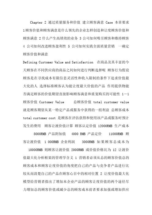
Chapter 2 通过质量服务和价值建立顾客满意 Case 本章要求1顾客价值和顾客满意是什么领先的企业怎样创造和让度顾客价值和顾客满意 2什么产生高绩效的业务 3公司如何吸引顾客和维持顾客4公司如何改进顾客盈利性 5公司如何实践全面质量营销一确定顾客价值和满意Defining Customer Value and Satisfaction 在商品及其丰富的今天顾客在不同供应商的商品之间如何进行判断选择呢顾客行为假设顾客是在寻找成本有限信息灵活性和收入限制的条件下追求价值最大化的人选择标准顾客认为能让度最大价值的产品作用提供物能否满足顾客的价值期望直接影响顾客满意和重复购买的可能性 1-1顾客价值Customer Value 总顾客价值 total customer value 就是顾客期望从某一特定产品或服务中获得的一组利益总顾客成本total customer cost 是顾客在评估获得和使用该产品或服务时预计发生的费用顾客让渡价值计算顾客认定价值 12000RMB 生产成本8000RMB 产品附加值4000 RMB 产品定价11000RMB 顾客让渡价值 1 000RMB 企业利润3000RMB 如果顾客总成本为10000RMB 则顾客让渡价值 2000RMB 或价值价格比为12 让渡价值最大化分析框架的管理学含义 1营销者必须从总的顾客价值总的顾客成本和顾客让度价值的角度把自己的产品与竞争者产品进行比较从而清楚自己的产品在顾客心目中的相对位置 2让度价值最大化模型给营销者指出了增加本企业产品的顾客让度价值的两个途径尽力增加总的顾客价值或减少总的顾客成本前者要求加强或增加供应物的产品服务人员和或形象利益后者要求减少购买者的成本 1-2顾客满意Customer Satisfaction 产品感知效果products perceived performance 产品感知效果是顾客在购买和使用产品之后依据自己的体验 resulting experience 所形成的对产品让度价值的认知顾客对产品的感知效果由顾客感知的让度价值来度量顾客感知的让度价值=顾客感知的总价值-顾客感知的总成本顾客期望Customer Expectation 满意与不满意顾客的消费行为 1不满意顾客往往是减少购买或转向其它供应商 2一般满意的顾客一旦发现有更好的产品依然会很容易地更换供应商 3十分满意的顾客一般不打算更换供应商因为高度满意和愉快创造了一种对品牌的情感上的共鸣而不仅仅是一种理性偏好正是这种共鸣创造了顾客的高度忠诚 loyalty Case 形成顾客忠诚的关键是向顾客让度更高的价值Simon Knox and Stan Maklan 1998 Competing on value bridging the gap between brand and customer value 价值缺口value gap =顾客价值-品牌价值顾客感知价值customer perceived value -品牌承偌价值brand promised value 顾客感知价值的水平由两个要素决定价值建议 value propositions 价值让度系统 value-delivery system 让度和使顾客感知品牌承偌价值的水平由两个要素决定品牌开发和品牌形象承偌的价值建议企业的核心过程实现价值承偌在企业资源的约束下企业在提供给其它利害关系者 stakeholders 至少接受的满意水平的基础上尽力提供一个高水平的顾客满意在顾客满意调查中存在的陷井 1营销者在调查之前讨好将被调查的顾客 2营销者在调查中有意排除不满意者 3顾客有意在调查中表达不满意以便获得企业方面的让步 2-4组织和组织文化 Collins and Porras 1994 Built to last Successful Habits of Visionary Companies 从18个行业中每个行业选两个企业一个成为有远见的企业另一个是对比企业其中选择有远见的企业得到标准是行业领导广泛赞誉有远大的目标把这些目标传播给员工拥有除了盈利以外的高意图high purpose 盈利超过对比企业有远见企业的共同特点 1每个企业有自己特定的价值观念 IBM尊重个人顾客满意持续改进质量JJ第一对顾客负责第二对员工负责第三对社会负责第四对股东负责2用启迪性的词汇表达企业的目的 Xerox改善办公室效率 3制定企业的远景规划并采取行动实现它 IBM作为网络中心型企业的行业领导三让渡顾客价值和满意Delivering Customer Value and Satisfaction Hammer and Champy Reengineering the Corporation 他们指出企业可以重组企业的业务建立跨部门团队来管理核心业务过程以便产生高水准的顾客价值其中企业的核心业务过程一般包括新产品实现库存管理顾客获得和维持从接受订货到回款的过程顾客服务 3-2价值让渡网络Value-Delivery Network 四吸引与保持顾客Attracting and Retaining Customers 企业除了改进与它供应链的伙伴的关系之外还试图与最终顾客建立紧密的纽带和忠诚关系 1吸引顾客 attracting customer 2计算流失顾客的成本为什么顾客维持及其重要 3顾客维持的需要 The need for customer retention 4关键关系营销 Relationship Marketing 5增加财务利益 adding financial benefits 6增加社会利益 adding social benefits 7增加结构性联系 adding structural ties 4-1 吸引顾客Attracting Customer 寻求成长的企业花相当多的时间和资源来寻找新顾客获得新顾客需要三个方面的技能 1发现潜在顾客lead generation 2甄别潜在顾客 lead qualification 3转化潜在顾客 account conversion 4-2计算流失顾客的成本为什么维持顾客及其重要某大运输公司是这样来估算其顾客流失成本的该公司有64000个客户今年由于服务质量差该公司丧失了5的客户也就是3200个客户005×64000 平均每流失一个客户营业收入就损失40000美元所以公司一共损失128000000美元营业收入3200×40000 该公司的盈利率为10该公司这一年损失了12800000美元利润010×128000000随着时间的推移公司的损失将更大降低顾客流失率的4个步骤 1确定和衡量它的顾客保持率例如杂志续订率大学一年级升至二年级的比率或者毕业率 2找出导致顾客流失的原因并找出那些可以改进的地方 3估算一下当它失去这些不该失去的顾客时所导致的利润损失当一个顾客流失时损失的利润就相当于这个顾客的生涯价值也就是说相当于这位顾客在正常年限内持续购买所产生的利润 4计算降低流失率所需要的费用只要这些费用低于所损失的利润公司就应该花这笔钱当顾客流失时应该自问的几个问题今年顾客流失的变动率是多少在各业务单位地区销售代表或分销商上的顾客保持率变化如何顾客保持率与价格变化之间的关系在流失的顾客上发生了什么和他们去向何方你所在行业的顾客保持率标准是多少在同行中哪一家公司顾客维持时间最长 4-3顾客维持的需要 A吸引一个新顾客所耗费的成本大概相当于维持一个现有顾客成本的5倍因为它需要耗费更多的精力和费用去劝导那些满意的顾客从他们目前的供应商那儿转换到本公司 B平均每年企业流失10%的顾客 C一个企业如果将其顾客流失率降低5依据不同的行业利润就能增加25至85 D在顾客维持期间内随着时间的增长顾客对企业的利润贡献也增大假设平均每次销售访问的费用300美元包括工资佣金津贴和其他开支使一个潜在顾客转变为现实顾客平均所需的访问次数×4 则吸引一个新顾客的费用 1200美元这个数字是低估的因为我们没有把广告促销营运计划等发生的费用计算在内〕假设公司对平均的顾客生涯价值CLV 估计如下平均来自顾客的年销售收入 5000 美元顾客平均的忠诚年限×2 公司销售毛利为×010 则顾客生涯价值 1000美元为什么顾客满意 CS 这么重要一个高度满意的顾客的消费行为特点忠诚公司更久购买更多的公司新产品和提高购买产品的等级对公司和它的产品说好话忽视竞争品牌和广告并对价格不敏感向公司提出产品服务建议由于交易惯例化因而对其的服务成本低于新顾客处理顾客抱怨的意义顾客满意的另一面测试顾客满意度高度满意一般满意无意见有些不满意极端不满意方便顾客投诉1〕95%左右的不满意顾客不会投诉它们中的大多数是停止购买2〕3M公司说它的产品改进主意的23来自顾客的意见对投诉作出具体反应如果投拆得到解决大约54~70的投诉顾客还会再次同该企业做生意如果顾客感到投诉得到很快解决数字会上升到惊人的95顾客对该组织投诉得到妥善解决后他们每人就会把处理的情况告诉5个人 LLBean LLBean 保留顾客途径Two ways to strengthen customer retention1设置高的转换壁垒 to erect high switching barriers 2提供高的顾客满意 to deliver high customer satisfaction 和建立顾客忠诚 to build customer loyalty 企业努力的方向〕--关系营销的任务 4-4关系营销对顾客关系进行类型Five levels of customer-relationship 基本型 Basic marketing 推销员只是简单地出售产品反应型 Reactive marketing 推销员出售产品并鼓励顾客如有什么问题或不满意就打电话给公司负责型Accountable marketing 推销员在售后不久就打电话给顾客以了解产品是否与顾客所期望的相吻合推销员从顾客那儿征集各种有关改进产品的建议以及任何不足之处这些信息有助于企业不断改进它的产品主动型Proactive marketing 公司推销员经常与顾客电话联系讨论有关改进产品用途或开发新产品的各种建议伙伴型Partnership marketing 公司与顾客互动协商以找到节省顾客花费或帮助顾客更好地行动的方式不同类型顾客关系的应用环境如何开发牢固的顾客纽带和让顾客满意建立顾客价值Customer Value-building Approaches 贝利和帕勒苏拉门 Berryand Parasuraman 1991 提出了3种建立顾客价值强化顾客关系的方法增加财务利益adding financial benefits 增加社交利益adding social benefits 增加结构性联系 adding structural ties4-5增加顾客的财务利益公司可用两种方法来增加顾客的财务利益A频繁营销计划 Frequency marketing programs 频繁营销计划 FMPs 就是设计向频繁购买和或大量购买的顾客提供回报和奖励频繁营销计划体现出一个事实20的顾客占据了80的公司业务如购买点数卡数量或数额折扣 B俱乐部营销计划 Club marketing programs 俱乐部成员可以因其购买自动成为会员也可以通过购买一定数量的商品入会或者付一定的会费企业对会员提供一定的优惠服务 Case Case 4-6增加顾客的社交利益adding social benefits 企业的员工针对每个顾客的需求和爱好通过定制化的服务把与顾客的关系个性化和人性化从而增加企业与顾客的社交纽带从本质上说关系营销者力图把它们的顾客变成了客户唐纳利贝利和汤普森描述了两者的差别 4-7增加结构性联系adding structural ties 公司可以向顾客提供某种特定设备或计算机联网以帮助客户管理他们的订单工资存货等等以便增加客户的利益同时增大顾客依附于企业而存在的专有性资产五顾客盈利性最终测试 Kotler 营销是一门吸引和维持有利可图顾客的艺术Marketing is the art of attracting and keeping profitable customers 根据美国运通公司总裁Putten的看法最好顾客的花费与其它顾客的花费比率如下在零售业为161在餐饮业为131在航空业为121在汽车业为51 根据著名汽车经销商Sewell估计一个典型的汽车消费者在汽车购买和服务方面的潜在顾客生涯价值为30万美元盈利顾客和亏损顾客著名的8020规则认为在顶部的20顾客创造了公司80的利润威廉·谢登 William Sherden 把它修改为802030规则其含义是在顶部的20顾客创造了公司80的利润但其中的一半的利润被在底部的30非盈利顾客丧失掉了哪些顾客能带来大的利润购买量大的顾客常常相求相当多的服务和很大的价格折扣从而减少了公司的获利水平购买量小的顾客支付全价服务也少但是交易时间和费用大中等规模的顾客能接受良好的服务支付的价格接近全价常常是最有利可图的顾客群有所为有所不为一些组织力图去做顾客所提出的任何事和每一件事但是在顾客经常提出许多好建议的同时他们也会提出许多无法操作或无利可图的行动建议盲目地采纳这些建议会严重背离市场导向原则确定一个明确的选择原则即应为哪些顾客服务以及向他们提供什么样的利益和价格组合和那些是应该拒绝的兰宁和菲利普 Lanning and Phillips什么样的顾客有利可图六实施全面质量营销按通用电气公司董事长约翰·韦尔奇 John F Welch Jr 的说法质量是我们维护顾客忠诚最好的保证是我们对付外国竞争最有力的武器是我们保持增长和盈利的唯一途径质量 Quality质量满意盈利的关系国家质量奖国家质量奖营销经理责任营销经理在一个以质量为中心的公司里有两项责任营销经理必须参与制定旨在帮助公司通过全面质量管理并获胜的战略和政策营销经理必须在生产质量之外传递营销质量每项营销活动营销调研推销员培训广告顾客服务等等都必须高标准地执行营销人员责任营销者在正确识别顾客的需要和要求时承担着重要责任营销者必须将顾客的要求正确地传达给产品设计者营销者必须确保顾客的订货正确而及时地得到满足营销者必须检查顾客在如何使用产品方面是否得到了适当的指导培训和技术性帮助营销者在售后还必须与顾客保持接触以确保他们的满意能持续下去营销者应该收集顾客有关改进产品和服务方面的意见并将其反映到公司各有关部门追求全面质量营销战略越来越多的公司已经任命一位质量副总经理专门负责全面质量管理TQMTQM要求确认下面有关质量改进的诸条件 The End 顾客维持和顾客忠诚的作用对企业长期盈利的贡献信用卡行业资料来源Reichheld 1994 pp241 顾客维持率%〕平均顾客维持年数年犹豫顾客不合格者首次购买顾客重复购买顾客预期顾客成为停止购买或以前的顾客客户拥戴型客户合伙人发展顾客过程吸引和维持顾客的过程〕会员型客户 suspects prospectsDisqualified prospects First-time customers Repeat customers clients members advocates partners Inactive or ex-customers Griffin 1993 Raphel 1995 顾客类型特征 1犹豫顾客 2预期顾客2不合格者 3首次购买顾客 4重复购买顾客 5客户 6会员型客户 7拥戴型客户 8合伙人 9成为停止购买或以前的顾客可能购买该企业产品和服务的任何人对该产品有强烈的兴趣且有支付能力的人或信用低或无利可图的被企业拒绝的人企业非常特别非常用心对待的顾客享受俱乐部套餐优惠的会员热情向别人推荐企业和该企业产品的顾客主动与企业在一起工作的顾客顾客分销商很多顾客分销商数量中等顾客分销商很少高利润中等利润低利润负责型负责型负责型主动型主动型反应型基本型反应型伙伴型边际利润水平顾客或分销商的数目今天最好的关系营销活动由技术来推动 DELL用WEB技术进行定制营销 e-mail Web sites Call center databases soft 双向沟通美国航空公司是首批实行频繁营销计划的公司之一80年代它决定对它的顾客提供免费里程信用服务接着旅馆也采用了这种计划马里奥特推出荣誉贵宾计划常住顾客在积累了一定的分数后就可以享用上等客房或免费房很快地汽车租凭公司也推出频繁营销计划尔后信用卡公司开始根据信用卡的使用水平推出积点制例如西尔斯公司为它的发现者卡持卡人在购买某些商品时提供折扣资生堂是日本一家化妆品公司该公司的资生堂俱乐部吸收了1000多万名会员该俱乐部给会员提供一个VISA信用卡提供戏院旅馆和零售店的折扣优惠还有老主顾分数俱乐部成员可以得到一本免费杂志里面有各种有关美容方面的文章对于某个机构来说顾客 customer 可以是没有名字的而客户 client 则不能没有名字顾客是作为某个群体的一部分为之提供服务的而客户则是以个人为基础的顾客可以由企业的任何人为其服务而客户则是指定由专人服务的与顾客建立良好社交关系的方法与顾客建立较差社交关系的方法主动打电话作出介绍坦陈直言使用电话力求理解提出服务建议使用我们等解决问题的词汇发现问题使用行话短话不回避个人问题讨论我们共同的未来常规反应承担责任规划未来仅限于回电作出辩解敷衍几句使用信函等待误会澄清等待服务请求使用我们负有等法律词汇只是被动地对问题作出反应拿腔作调回避个人问题只谈过去的好<a name=baidusnap0></a>时光</B> 救急紧急反应回避责难重复过去影响买卖双方关系的社交行动著名的药品批发商麦肯森公司 Mckesson 在该方面就是一个很好的例子公司在电子数据交换EDI方面投资了几百万美元以帮助那些小药店管理其存货订单处理和货架等另一个例子是米里步公司 Milliken 向它的忠诚顾客提供运用软件程序营销调研销售培训和推销指导等为公司带来最大利润的并不是最大的顾客一个有利可图的顾客就是指能长期持续产生收入流的个人家庭或公司其收入流应超过企业吸引销售和服务顾客所花费的成本流即顾客生涯价值较大的顾客 P1 P2 P3 P4 高盈利产品盈利产品亏损产品无利润产品 C1 高盈利顾客 C2 - 无利润顾客 C3- - 亏损顾客产品顾客顾客产品盈利性分析工具〕或提高P3或P4的价格或只向其销售P1产品或今后终止与其交易企业创造价值能力越大内部运作越有效竞争优势顾客优势越大获利水平越高顾客期望从销售者得到的主要价值之一是高质量不是平均质量的产品和服务企业管理者的任务是应用 TQM改进产品和服务的质量让顾客完全满意全面质量管理 TQM 是持续不断地改进所有组织过程产品和服务的质量的一种全企业范围的管理方法质量是产品或服务所具有的满足人们需要的特性和特征的总和一致性质量Conformance quality 与目标顾客的需要和期望相吻合性能质量 Performance quality 指产品本身所具有的性能状态适应性质量符合性质量顾客满意企业盈利较高的价格较低的成本高的质量日本1951年日本第一个设立国家质量奖戴明奖美国80年代中期美国设立了以已故商务部长命名的麦尔肯·鲍特里奇国家质量奖该然由7个衡量标准组成每个标准含若干奖励分数顾客为中心和满意得分最多质量和营运结果管理过程质量人力资源开发与管理战略质量计划信息和分析高层经理领导欧洲为了参与质量竞争欧洲在1993年设立了欧洲质量奖该奖由欧洲基金会为质量管理和欧洲质量组织专门设立类似于鲍特里奇奖它奖励在下面领域取得高分的公司领导层人员管理政策与战略资源生产过程员工满意顾客满意社会影响业务结果欧洲质量奖的发展后来与另一个国际质量标准密切相关这就是ISO9000它是一整套的对质量进行文件式管理的方法并被普遍接受ISO9000提供了一套框架以体现在世界范围内顾客对质量导向的态度员工训练记录保存确定不足之处等问题获得ISO9000证书需要由国际标准化组织认可的质量评估师每半年一次的认证核心能力的特点Characteristics of core competence 1能带来竞争优势地位 2有较为广泛的应用宽度延展性 3能带给顾客高的附加价值 4具有独特性专有性不易模仿accrue 能带来竞争优势地位企业的核心能力能带来竞争优势地位是其区别于其它基本能力的必要条件反过来说如果核心能力不能带来竞争优势地位则就不能称之为核心能力有较为广泛的应用宽度延展性企业核心能力必须具有应用上的广度即在多个领域为企业带来竞争优势核心能力光学镜片成像技术微处理控制技术终端产品复印机激光打印机照相机扫描仪传真机等 20多个领域佳能公司核心能力 LCD 液晶技术终端产品笔记本电脑台式电脑摄像机液晶电视机液晶背投式电视机夏普公司能带给顾客高的附加价值核心能力能真正满足顾客的核心需求带给顾客高的附加价值区别核心能力与非核心能力的标准之一是它是否带给顾客所需要的核心利益发动机传动系统节省汽油启动方便加速迅速噪音低振动小提供的利益核心能力顾客核心价值本田公司顾客认知具有独特性专有性不易模仿核心能力必须具有独特性和专有性这样才能不易被竞争对手占有转移或模仿从而企业才可以维持由核心能力所带来的竞争优势如本田的传动系统在过去的20年时间维持了专有性竞争对手不易模仿所以建立和维持独特的核心能力是企业获得长期竞争优势的源泉企业组织组织结构组织政策组织文化依环境的变化能改变虽然较为困难〕非常困难所以改变企业文化常常是成功执行新战略的关键大学合并公司文化体现组织特征的在组织内部共享的经验历史信仰和行为标准 the shared experience stories beliefs and norms that characterize an organization CASE 微软如果一个公司像一辆汽车那么它不应该有后窗微软公司的副总裁马克·默里说他负责人力资源和管理微软并不对过去的成绩沾沾自喜公司的文化表现出向前看和企业的精神但令人奇怪的是这里并没有人意识到要分享它的文化大多数微软的员工年龄在30岁左右这是受公司文化强烈影响的一代人的确微软像一个大学校园员工衣着随便互相称呼名而不是姓自由地谈论自己的思想但这都是表面现象微软员工在新产品开发上特别卖力地工作每个员工每半年评定一次工资和奖金全世界没有一家公司像微软那样有那么多的百万和亿万收入的员工价值链工具价值让度网络如何产生价值如何让度价值支持活动 support activities 公司的基础设施人力资源管理技术发展采购运入生产运出营销与服务物流操作物流销售基础活动primary activities 3-1价值形成链和成本形成链价值链为企业评价每个价值创造活动的成本和绩效以及寻找改进价值创造活动的方法提供了一个分析工具用定点超越法benchmarks 比较竞争者在每个价值创造活动中的成本和绩效发现比竞争者做得更好的改进方。



2.DYNAMIC EQUILIBRIUM MODELS I:TWO-PERIOD ECONOMIESInterest always carrieth with it an ensurance praemium.–Sir William Petty(1623–1687)To be able to study intertemporal prices(interest rates)or plans for behaviour over several periods,as well as growth,we need a dynamic,equilibrium model.The simplest dynamic models have two periods and that is where we begin.(a)Exchange EconomyMacroeconomics is about dynamics,and about how the different decisions made by consumers andfirms–saving,investment,employment,and so on–interact.We shall next look at some of these decisions,and the resulting equilibrium,in the simplest possible dynamic economy:a two-period,single consumer,exchange economy.The idea,which dates back at least to Irving Fisher,is to look at the allocation of goods over time the same way we treat the allocation of resources to different goods at a point in time.We simply treat goods at different dates as different commodities.The essential elements of our dynamic economy are:(a)The list of commodities:consumption now(c1)and later(c2).(b)Endowments of the commodities,y1and y2,which are nonstorable.(c)The preferences of a single‘representative’consumer,characterized by the concave utility function u(c1,c2).(a)and(b)summarize the feasible allocations of this economy,namely c t≤y t,for t=1,2. There is no uncertainty in this environment;we’ll allow for that later.This summarizes the environment.The question is how the consumer behaves and what determines prices and quantities,the objects of interest.One theoretical assumption which is simple and the implications of which are testable is that the agent operates in a system of competitive markets.The goods,consumption now and later,sell at prices p1 and p2,respectively.The consumer is endowed with quantities y1and y2,respectively,of the two goods and maximizes utility subject to the budget constraintp1c1+p2c2≤p1y1+p2y2and prices adjust so that,in equilibrium,supply and demand for each good are equal.In other words,we define a competitive equilibrium as a price system{p1,p2}and allocation{c1,c2}such that:(a)the consumer maximizes utility subject to the budget constraint for given prices;and(b)(feasibility)supply equals demand for each good:c t=y t for t=1,2.Let us take an example that we can solve explicitly.Suppose utility isu(c1,c2)=ln c1+βln c2forβ>0.We shall use log preferences frequently.Typically we’ll choose0<β<1, implying that consumers discount future consumption relative to current consumption.It takes more than one unit of future consumption to compensate the agent–in the sense of maintaining the level of utility–for the loss of one unit of current consumption at any point along the ray c1=c2.[Graph the isoquant,showβas the slope along the45◦line.] Sometimes we shall write U for the lifetime utility function and u for the period utility function.With this notation we have U=u(c1)+βu(c2),u(c)=ln c.Wefind the equilibrium as follows.First,the consumer maximizes utility subject to the budget constraint.This yields the“demand functions”c1=11+βy1+p2p1y2c2=β1+βp1p2y1+y2Now we impose the second part of the definition of equilibrium,that supply equals demand. Note that both conditions,c1=y1and c2=y2,produce the same result:p2/p1=β(y1/y2). At these prices the allocation is,obviously,c t=y t.This brings us to an important point about exchange economies that sometimes is con-fusing.We work with these models because they are simple;in particular the consumption allocation can be read offfrom the endowments,because the good is perishable and cannot be stored or invested.But if people cannot save why do we write down a multiperiod bud-get constraint and how is an interest rate or intertemporal relative price determined?A practical notefirst.To solve these modelsfirst work out the household planning problem in general,then use the technology and equilibrium conditions to determine the allocation and prices.Second,one can think of this two-period model without storage as an auction. At the beginning of time the auctioneer can deduce the relative values people attach to c1and c2by offering them trades between the goods at different dates.If people value c1 more than c2then p1will exceed p2,for example.Thus the relative prices tell us some-thing about people’s impatience or willingness to substitute between the two periods,even if they are not able to do so on their own if there is no storage or investment.And this result will continue to apply in more realistic models.There,as we shall see,the interest rate or intertemporal relative price tells us about investment possibilities,but it also tells us about people’s preferences,a fact illustrated most simply in the endowment economy.As a rule,the definition of equilibrium only determines relative prices,here p2/p1,not prices themselves.If we multiply p1and p2by a positive constant the new prices are also an equilibrium for the same allocation.Thus we are free to choose one price arbitrarily, say p1=1.In this case all prices are measured in units of thefirst good.The price p2 then means that one unit of consumption tomorrow costs p2units of consumption today.Thus,the allocation{c1=y1,c2=y2}and prices{p1=1,p2=β(y1/y2)}constitute a competitive equilibrium for this economy.Now one of the things we know about competitive equilibria in such economies(in fact,for a large class of economies)is the fundamental theorems of welfare economics: competitive allocations are Pareto optimal,and optimal allocations can be supported as competitive equilibria.Given the resource constraints on the economy,no consumer’s utility can be increased without lowering someone else’s.(This is the sense in which com-petitive markets are said to produce an efficient allocation of resources.)In this economy there is a single agent,and thus no difficulty of comparing utilities across them and no sense in which distribution matters for macroeconomic properties.A Pareto optimum is an allocation{c1,c2}that maximizes utility subject to the economy’s resource constraints, c t≤y t.The solution to this problem is,obviously,for the representative agent to consume the entire endowment,c1=y1and c2=y2,so we have verified thefirst welfare theorem for this economy(the competitive allocation derived above is the same).Moreover,the relative price implicit in this allocation can be computed from the marginal rate of substi-tution.The mrs between the two goods is the ratio of the marginal utility of consumption tomorrow to the marginal utility of consumption today,with both derivatives evaluated at equilibrium or optimum quantities:mrs=(β/c2)/(1/c1)=β(y1/y2).Thus p2/p1=mrs=β(y1/y2)as before.[Practice:derive p2/p1=(du/dc2)/(du/dc1)= mrs from the consumer’sfirst-order conditions.]It is sometimes convenient,in model economies to which the welfare theorems apply, to compute a competitive equilibrium by solving a welfare maximization,rather than going through the consumers’problem and imposing the market clearing conditions.Exercise3 illustrates this point in a related two-person economy.We have,to this point,done little to distinguish this dynamic economy from a static one with two goods,haggis and oatcakes,say.There has been no mention of the rate of interest,for example.Consider,then,a slight change in notation in which the intertemporal character of the economy is made more explicit.We can think of our consumer as deciding, in thefirst period,how much to save:choosing,that is,s=y1−c1.In the second period the agent takes the proceeds from saving,after interest,plus second-period income,and spends it:c2=(1+r)s+y2,where r is the rate of interest paid on saving.The consumption-saving decision clearly has an intertemporal character to it.In equilibrium the rate of interest equates supply and demand:c t=y t.Note that r is a real,or commodity,rate of interest,since it is measured in units of goods:goods tomorrow for goods today.Thus the rate of interest is defined by1/(1+r)=p2/p1=β(y1/y2).If y1=y2this takes a particularly simple form.The discount factorβis often expressed in terms of a discount rateθ,withβ=1/(1+θ).When y1=y2,the equilibrium interest rate is r=θ.In general the interest rate depends on both the discount factor and the endowments.We usually think of r as being positive(reflecting,in this last,steady-state example, impatience).Since1+r=p1/p2that means that p1>p2.The endowment at time1 commands a higher price since no waiting is involved.It may seem odd that the interest rate is determined,since the economy as a whole does no saving in equilibrium.But consumers can still value marginal units of the endowments and hence determine a relative price. (Try drawing a picture of this).If you have studied interest rates before,then you might be thinking:This r is simply a commodity own-rate or real rate of interest.So shouldn’t rises in the price(p2>p1) correspond to positive interest rates?In fact,this way of thinking is correct.Let us clarify the units in which these prices are quoted:p1 p2=utility per goods todayutility per goods tomorrow =goods tomorrowgoods today=1+rFor future reference,suppose that prices are quoted in money terms.Let P denote the good’s price in dollars.ThenP2 P1=$per goods tomorrow$per goods today =1+πwhereπis the inflation bining these two results,p1 p2·P2P1=(1+r)(1+π)=goods tomorrowgoods today·$per goods tomorrow$per goods today =$tomorrow$today=1+Rwhere R is the nominal interest rate.(b)Production EconomyOurfirst theoretical economy was an exchange economy,by which we mean that there was no opportunity for producing goods–consumers simply exchange what is available in competitive markets.In that economy the rate of interest is determined by the represen-tative consumer’s preferences for present and future consumption,including the discount factorβand the endowments y1and y2.More generally the rate of interest will depend,as well,on the technological opportunities for transforming current consumption into future consumption.For example,if the endowment y1is storable and a unit stored at time1 yields(1+g)units at time2then the interest rate will be g(show this).More generally,consider the possibility of investment in physical capital.We shall say that k units of investment leads to f(k)extra units of the good next period;if we set aside k units in period1we can have k(1−δ)+f(k)units in period2.Hereδis the rate of depreciation of the capital stock.We assume that the following conditions apply to the function f:(i)No investment,no extra output:f(0)=0.(ii)f is increasing and concave: f >0,f <0.(iii)The Inada conditions,f (0)=∞and f (∞)=0.[Graph f(k)vs k and show how the conditions apply.Show that the marginal rate of transformation is the slope of the production possibilities frontier.]The possibility of production introduces another actor into the economy,afirm which buys(or rents)capital from consumers at price q per unit and uses it to produce extra output in the second period.Thefirm chooses the amount of capital to maximize profit:PR=p2[k(1−δ)+f(k)]−qk.[Graph this vs k,show that there is afinite interior maximum(due to the Inada condi-tions).]q is the price of capital.The representative consumer owns both the capital stock and thefirm,and her budget constraint changes as follows.Let x be the amount of capital rented tofirms and PR be profits from owning thefirm.Then the consumer chooses consumption quantities,c1and c2,and capital rentals x to maximize utility subject to the budget constraintp1c1+p2c2≤p1(y1−x)+p2y2+qx+PR.Clearly we must have p1=q in equilibrium(or the consumer would choose x equal to plus or minus infinity).In this expanded economy the definition of equilibrium changes as follows.The list of commodities is{c1,c2,x,k}.A competitive equilibrium is a price system{p1,p2,q}and allocation{c1,c2,x,k}such that:(a)the consumer maximizes utility given prices and subject to the budget constraint;(b)thefirm maximizes profits given prices and technology;and(c)supply equals demand for each good:c1+k=y1,c2=y2+k(1−δ)+f(k),x=k.The definition of a Pareto optimum also changes.An optimum in this economy is an allocation that maximizes the utility of our representative agent,U(c1,c2),given the en-dowments and technological possibilities of the economy:subject,that is,to the feasibility constraintsc1+k≤y1,c2≤y2+k(1−δ)+f(k).[Graph the production possibilities set.]Again,the optimum problem often provides a shortcut tofinding a competitive equilibrium.Notice that the planning problem involves no prices.Let us again turn to a concrete example.Let u=ln c1+βln c2,as before;y1=y and y2=0;and f(k)=kα,with0<α<1.Also assume thatδ=1so that there is100% depreciation.It is convenient to substitute the feasibility constraints into the objective function,giving us the optimum problem,max ln(y−k)+βln(kα).Thefirst-order condition is:−1 y−k +βαkα−1kα=0which impliesk=(αβ1+αβ)y.In short,a constant fraction of thefirst-period endowment y is saved(this is a result of using log utility),and used to produce output next period.The consumption decisions are readily derived from the resource constraints:c1=y−k=(11+αβ)y,c2=f(k)=(αβ1+αβ)yα.Thus the optimal allocation,{c1=(1−ω)y,c2=(ωy)α,k=ωy},forω=αβ/(1+αβ), depends on preferences(throughβ),technology(α),and the endowment(y).Prices.It is clear,first,that in any equilibrium we will have q=p1(in a sense,both prices pertain to the same good).We canfind the relative price p2/p1=p2/q from either the marginal rate of substitution or the marginal rate of transformation.Thefirst gives usp2 p1=mrs=β/c21/c1=β(1−ω)yωyα,the secondp2 p1=mrt=1f (k)=ωyα(ωy)α.These reflect,respectively,thefirst-order conditions of the consumer and thefirm.[Prac-tice:Verify these relations for the general case.]Notice that afirst-order condition forprofit maximization is(1−δ)+f (k)=p1p2=1+r,f (k)=r+δ.One can think of the interest rate r=p1/p2−1as reflecting either impatience or produc-tivity.From the marginal rate of transformation,if there is a storage such that investing 1at time1yields1+g at time2then r=g.In the example above investing k at time 1yields k(1−δ)+f(k)at time2so that investing an additional unit at time1yields f (k)+(1−δ)at time2.Thus in the example the interest rate is r=f (k)−1because δ=1.In this notation we assume that one gets back the original investment(i.e.that f is a net rather than gross production function,so that its marginal product is the net rather than gross interest rate).Incidentally,you should be able to verify that solving this simple example would be much more difficult had we not assumed100%depreciation.For more realisticδ’s, numerical methods might be used.A lot of macroeconomics can be done with the two-period models we have seen so far in this section.Aside from adding more periods(which we won’t do explicitly)there are at least two obvious extensions:allowing for leisure and elastic labour supply,and adding a government sector.We’ll make these additions in applications below.To make these extensions interesting we also need to introduce some uncertainty in these two-period economies.So far we have assumed that when decisions are made in period1the values of period-2exogenous variables are known.(c)Uncertainty and ExpectationsTo make progress in introducing some realistic uncertainty we shall assume that it can be described by standard tools of probability.The randomness or uncertainty arises from exogenous variables which can take on one of several different values.In the two-period economy a good example of such a variable is the exogenous endowment{y1,y2}.Other examples might include tax rates,the money supply,or some property of the production function(i.e.there might be lean years and fat years).As a simple stationary example suppose in the endowment version that{y1,y2}have the following joint density:Outcome Probability(1,1)0.3(2,1)0.2(1,2)0.2(2,2)0.3which is a valid density because the probabilities sum to one.This is the simplest example because there are only two possible outcomes.More generally we might think of modellingwith continuous random variables,but this way we can calculate means and variances bysimple addition.Next we shall assume that agents know that the realizations of income are draws fromthis urn.Assuming that they know the true urn is sometimes called the hypothesis ofrational expectations–more on this in section3.Thus when we speak of their expectationsof y2,for example,we identify those with the actual mathematical expectation from thisprobability density function.What is E(y2)?We know that y2can take on two values:1and2.Tofind theprobabilities attached to these we need tofind the marginal density of y2.It is easy to seethat Prob(y2=1)=.5and Prob(y2=2)=.5simply by summing the cases from the jointdensity in which y2takes on each value.Thus E(y2)=1.5.This is sometimes called theunconditional expectation.However,in this example y1occurs before y2does.One obvious property of the jointdensity is that states tend to be persistent.If y1is low then y2is more likely to be low thanhigh,and conversely.Thus is a realistic feature of business cycles;periods of low incomeare likely to follow periods of low income and there is some persistence or autocorrelationto deviations from trend.But that fact built into this example suggests that agents can improve their forecastof y2if they observe y1,simply because the two random variables are not independent.Once period1events occur agents can condition on them.The conditional forecast orexpectation is denoted E1y2to show that it is the expectation based on information knownabout period1.An alternative notation which is often clearer is E(y2|y1)which shows precisely what variable in period1can be used to help forecast y2.To calculate thisexpectation we again use the two possible outcomes for y2but now weight them by theconditional probabilities.Conditional probabilities are given by dividing joint by marginal.So if we are instate1in period1then Prob(y2=1|y1=1)=.3/.5=.6and Prob(y2=2|y1=1)=.2/.5=.4.Thus E(y2|y1=1)=2·.4+1·.6=1.4.This is lower than the unconditional expectation,as one would expect.Knowing that y1has taken a low value causes one to revise downward the expectation or forecast of y2.This reflects the fact that the two random variables are positively correlated.One could work out the covariance or correlation from the probabilities given;if it were zero then the conditional and marginal expectations would coincide.Now we are ready to introduce uncertainty in two-period models.We simply have tobe careful to specify joint distributions and then say what agents know or condition on attime1,or else to write down a conditional density directly.Think of this as an importantpart of the model.Take the endowment economy as an example.Now agents maximize expected utility.Suppose thatE U=E(ln c1+βln c2|y1)=ln c1+βE(ln c2|y1),and notice that the expected value of the log of a function does not equal the log of the expected value.We know in this economy that the allocation is c1=y1and c2=y2so let us study the interest rate.Afirst-order condition is1 c1=E[β(1+r)c2|y1].It may seem that we have differentiated through the expectations operator,which is not correct for nonlinear functions.But we now can show that this Euler equation is correct. To derive the Euler equation,suppose that the household knows the current state of theworld(y1)but that there are two possible states for the next period,y2and y2.Then thereare also two possible values for c2and,in general,for the interest rate.The budgetting problem now involves choosing c1and a plan for c2in each state.The plan consists of c2and c2.The idea is that we treat second-period consumption as two different goods, depending on the state which occurs.Let us assume in the example that the probability of the low state is0.6and of the high state0.4.Maximizing expected utility in the log example means:EU=log(c1)+β[0.6ln(c2)+0.4ln(c2)]subject toc2=y2+(1+r)(y1−c1)c2=y2+(1+r)(y1−c1)In problems like this it is best to use the sequence form of the budget constraint.Call the Lagrange multipliers on these two constraints(only one of which can end up applying)λandλ.Thefirst threefirst-order conditions are:1c1+λ(1+r)+λ(1+r)=0β0.6c2+λ=0β0.4c2+λ=0.Then putting these together gives1 c1=β[0.6(1+r)c2+0.4(1+r)c2]=βE1(1+r)c2,which confirms our result.The Euler equation links two endogenous variables:interest rates and consumption. The general version isu (c1)=E1[β(1+r)u (c2)].This makes intuitive sense.Suppose you are deciding how much to save.The cost of saving a bit more is the marginal utility of current consumption,because that is what you forego by saving.The benefit is that you can take a saved unit and invest it,earning(1+r) units next period.That benefit in goods is converted into utility terms by multiplying it by marginal utility then(u (c2)).Then the future utility benefit is discounted,so as to be comparable to today’s cost.To show that this uncertainty can make a difference let us look at a very specific type of interest contract,in which one invests1at time1and receives1+r at time2no matter which state occurs then.In that case there is no uncertainty about the return so we can take it outside the E operator:1 1+r =βc1E[(1c2)|y1].Jensen’s inequality holds that for a function which opens up,as the function y=1/x does, the expected value of the function is greater than the function of the expected value.Thus the right-hand side is greater thanβc1/E(c2).Therefore,in this economy the interest rate is lower than in an otherwise identical economy with the same average second-period consumption but lower variance in it.The intuition is that with uncertainty in future income(and with this utility function)people try to save more(this is sometimes called precautionary saving)and so they bid up p2relative to p1.Notice that the risk in this example is in income and not in the asset’s payoff.In a few pages we shall see the effect of payoffrisk too.In dynamic models agents may be uncertain about productivity or about aspects of government ter sections will provide some illustrations of the effects of such uncertainty.We’ll next outline two interesting applications of these two-period model economies. Further applications are found in later sections of the course.(d)Application:Labour Supply and Lucas’s CritiqueSo far our household has consumed but not worked.It is simple to add labour supply and demand to our two-period framework,though.In growth theory(section4)we shall often assume that labour is supplied inelastically: households have an endowment of time and they supply this in a labour market so they labour supply curve is vertical.The idea is that cycles in unemployment and participation rates can be ignored for long-run analysis.In that case,real wages depend on the size of the labour force and on the demand for labour.Exercise Suppose that in the two-period production economy the consumer has endowments y1=y and y2=0of the good,and endowment n2=1of labour in the second period.The consumer has log utility,as a function only of the two consumptions.There is100percent depreciation,and the production function isf(k,n)=kαn1−α.Solve for the real wage.As you can see from this exercise,changes in the real wage must come from shifts in the labour demand curve(or else changes in population or participation)in this environment. What explains a trend in real wages in developed economies?In business-cycle theory(section5),in contrast,we usually focus on the elasticity of labour supply.That is modelled by assuming that leisure enters the utility function.We won’t look at a general equilibrium example here,but simply study the agent’s labour supply decision.Consider a two-period model in which a representative agent has preferencesU=ln(c1)+ln(1−n1)+βln(c2)+βln(1−n2)where c is consumption,n is labour supply(hours worked),and hence1−n is leisure.Thebudget constraint isc1+c21+r=n1w1+n2w21+r,where w is the wage rate.We need not specify the production side or solve the general equilibrium.Instead we shall focus only on the household’s plans and incentives,so that we take wages as given.There is no uncertainty.Tofind the optimal plan,simply form the Lagrangean and solve for c1,c2,n1,and n2.Thefirst-order conditions are the budget constraint and1c1+λ=0βc2+λ1+r=0−11−n1−λw1=0−β1−n2−λw21+r=0Exercise:Eliminateλthree different ways,giving Euler equations which describe the choice between c1and c2,between c1and n1,and between n1and n2.Eliminatingλand substituting in the budget constraint gives:c1(2+2β)=w1+w2 1+r,so thatc1=12+2β[w1+w21+r]c2=β2+2β[w1(1+r)+w2]n1=1−12+2β[1+w2(1+r)w1].where wages,and the interest rate are taken as given by the bining Euler equa-tions and the budget constraint gives us the consumption function and the labour supply function.However,we often cannot solve for these explicitly when there is uncertainty. In the exercises,you’ll see that with uncertainty we usually need to restrict ourselves to some special cases of the utlity function(such as quadratic utility)in order to solve for the consumption function,for example.Two very general macroeconomic ideas show up in these decision rules.One is the permanent income hypothesis:consumption depends on the present value of labour income. We’ll study this idea in detail in section6.The other idea is intertemporal substitution.As usual,a quantity decision depends on a relative price,in this case relative wages in the two periods.You can see that if w2rises relative to w1then n1falls;labour supply in period2is substituted for labour supply in period1.Section5discusses some of the evidence for this effect.You might think that wages do not vary much from period,unless the comparison is between straight-time and overtime.One potential source of variation in the intertemporal prices which affect labour supply,consumption,and investment is government policy.For example,suppose that there is a taxτon wage income.Then the budget constraintbecomesc1+c21+r=n1w1(1−τ1)+n2w2(1−τ2)1+r,andfirst-period labour supply is:n1=1−12+2β[1+w2(1−τ2)(1+r)w1(1−τ1)].To isolate the effect of tax changes let us assume that w1=w2=w.Next,we can use the two-period model tofind the effect on labour supply of a policy change.Suppose that we want to see the effect of a tax cut(dτ1<0).It is natural to start byfinding dn1/dτ1 (it is negative).Why would we want to know this?The answer is that we need to predict the effects of the tax cut on tax revenue and on output.Tax revenue is here given by T1=τ1w1n1. Thus the effect on revenue is:dT1 dτ1=w1n1+τ1n1dw1dτ1+τ1w1dn1dτ1.Thefirst term is just the tax base,the third term seems to be given from our labour-supply decision rule,and the second term requires a general equilibrium model of the labour market(and not just the agent’s problem as outlined here).Usually one imagines that the total effect is positive.The Laffer curve graphs the case in which it may be negative at large values ofτ(as for cigarettes),which requires a very large labour-supply elasticity.That raises the question of how elastic labour supply is in reality.Perhaps。
