【免费下载】Exmaple5——contour plots over maps
- 格式:pdf
- 大小:362.89 KB
- 文档页数:10
tecplot使用手册大部分是根据tecplot 9.0写的,不过应该10。
0等等也差不多。
一、简介tecplot包含两部分,一部分是数据的组织方式,另一部分是软件的基本操作.tecplot9。
0的三维数据显示功能大大增强了。
数据的组织方式和显示有很大关系。
数据的组织分成I,IJ,IJK组织.I组织类似行向量按照自然顺序排列。
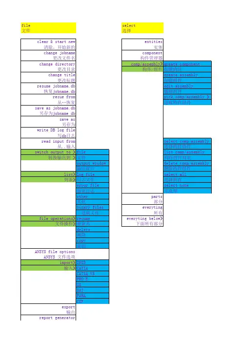
二、tecplot的菜单结构File,Edit,View,Axis(XY,2D,3D),Field,XY,Style,Data,Frame,Workspace,ToolsFrame modes有3D,用来表示表面、体积数据.2D表示2D field plots。
XY,S(ketch)。
layer有两种-——+zone layers,包括contour,vector等等.———+map layers,包括lines,symbols,bars等等。
针对XY—plotting。
针对的数据是XY方式组织的或者是I—ordered.三、tecplot的坐标系统包括:paper,frame,2D physical coord。
,3D physical coord.,paper左上角为原点.frame和2D,3D在左下角为原点.frame的长宽均为100.cell-centered data对于网格中心的数据,tecplot可以将其变换为网格节点上的数据。
可以通过Shift Cell-centered Data (Data menu)将其改变.Extract Data points可以有三种方法:——-+用鼠标选择离散点集——-+用鼠标画一个polyline,从某点开始———+用鼠标画一个geometry,从某点开始二进制数据格式比ASCII数据格式更快,因为他们占用更少的空间。
TECPLOT 的ASCII数据文件可以分成若干个RECORD:ZONE,TEXT,GEOMETRY,CUSTOM LABELS,这些RECORD排列在文件头后面。
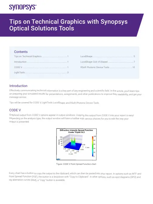
Introductio nEffectively com municating tec hnical informat ion is a key par t of any engine ering and scien tific field. In this article, you’ll le arn tips on preparing yo ur simulated re sults for presen tations, assignm ents, and other publications to improve their r eadability, and get your message acros s.Tips will be cov ered for CODE V, LightTools Lu cidShape, and R Soft Photonic D evice Tools.CODE VGraphical outp ut from CODE V options appea r in output wind ows. Copying t his output from CODE V into yo ur report is eas y! Depending on t he analysis typ e, the output w indow will have a toolbar with various choices for you to edit the way your output is presented.Figure: CODE V P oint Spread Func tion chartEvery chart has a button to cop y the output to the clipboard, w hich can then b e pasted into yo ur report. In op tions such as M TF and Point Spread F unction (PSF), t he button is a d ropdown with “Copy to Clipboa rd”. In other op tions, such as s pot diagrams (S PO) and ray aberration c urves (RIM), a “Copy” button is available.ContentsTips on Technical Graphics (1)Introduction (1)CODE V (1)LightTools ...........................................................................3LucidShape .........................................................................5LucidShape CAA V5 Based ..............................................7RSoft Photonic Device Tools .. (10)vFigure: Copying charts from CODE V’s MTF option and Spot Diagram optionAnalysis options such as MTF and PSF have buttons to increase font size and line width to aid you in making your output more legible when pasted into results. There is even an “Apply Presentation/Report Template” button to quickly prepare the chart for presentations:Figure: Controls to adjust chart font size, line width, and switch to “Apply Presentation/Report Template”Figure: MTF chart copied using the default MTF template (on left), and Presentation/Report settings (on right).Notice the text in the chart on the right is easier to read.For more extensive chart customizations, you can press the Chart Properties button to access controls for chart colors, axes scales, and more.Figure: Some options have a toolbar button to customize chart properties furtherRight click on the chart to save the property settings as a template to use later, or apply the settings to all similar charts in the window.Figure: Right clicking on a chart gives you options to apply and save templates,apply settings to all charts in the window, and revert settings back to the defaultFor charts that don’t have editable properties, such as spot diagrams and ray aberration curves, you can extract the components in Microsoft products and edit the picture:Figure: Copy of a RIM curve in Microsoft Powerpoint. Right click to edit the picture (left).Example of edited picture after adjusting font and line sizes (right)The edited picture becomes a Microsoft drawing object. These objects can then be ungrouped and moved/modified independently. LightToolsGraphical output from LightTools analysis can be accessed from the Analysis menu and choosing the metric you’d like to assess (illuminance, intensity, luminance, etc.). The main output is to present illumination metrics using the LumViewer, but there are also other types of analysis for color charts, polarization, and more. Each chart has a toolbar to help you customize how the analysis is presented.Copying charts from the LumViewer is easy! Right click on the copy icon and choose “Copy to Clipboard”. You can then paste the chart into your document.Figure: LumViewer’s “Copy to Clipboard”You can make text more readable by adjusting the font size up and down.Figure: In the LumViewer toolbar, you can adjust text font sizevFigure: Irradiance LumViewer plot copied with default settings (on left),compared to chart copied after increasing the font size to be more readible.For more extensive chart customizations, you can press the Chart Properties button to access controls for chart colors, axes scales, and more!Figure: Analysis options have a toolbar button to customize chart properties furtherRight click on the LumViewer to save the property settings as a template to use later, or apply the settings to all similar charts.Figure: Right clicking on a LumViewer chart gives you options to apply andsave templates and apply settings to all charts in the window.For luminance measurements, you can overlay forward simulation results directly on the associated geometry in the V3D window. To enable this setting, go to the View menu > Simulation Results and choose True Color or False Color.Figure: False color illuminance overlaid on lens geometry in the LightTools 3D ViewLucidShapeGraphical output from LucidShape can be customized from context menus for the specific output. After you’ve opened the results, you can customize the appearance by right clicking on the chart.Figure: Analysis from LucidShapeTo copy a chart or GeoView from LucidShape, right click in the window’s area and select “Copy Bitmap”. You can now paste the chart from the clipboard to the desired destination.Figure: To copy output from a chart or the GeoView, right click and choose “Copy Bitmap”You can use other options from the context sensitive menu as well. For example, when plotting sensor data you can switch ISO lines off for a smoother view, and select “View Properties” to open further chart customizations:Figure: For chart customization, right click and choose “View Properties”In the properties window, you can change settings such as the axes ranges, the type of chart, the scale, and more:Figure: The data properties windows lets you customize the way sensor data is presentedYou can customize the GeoView too! The context menu has choices to set the background color and edit the global axis system attributes the Stock Scene selection.• From the GeoView’s Options menu > GeoView, you can set the background color and edit stock sceneFigure: GeoView with the global axis system (on left) and without the stock scene visibleFrom the GeoView’s Options menu > Global Settings, you can increase the line widths to make wireframes clearer to see inpresentations and reports.Figure: Wireframe view with default width (on left) and increased line width (on right)The GeoView toolbar has options to change orientation and the change surface rendering mode. For instance, you can switch between shaded/wireframe modes, and even display sensor results from “Display Light Data”.Figure: GeoView with shaded geometry (on left), wireframe geometry (middle), and Display Light Data (on right) LucidShape CAA VA BasedTo take a screenshot in CATIA you can go to Tools > Image > Capture:Click the 3rd Icon “Options”:In the second tab “Pixel”, you can check “White background”, “Anti-aliasing” and switch render quality to “Highest”:Click OK, and back with these icons, click the second one “Select Mode”, and then do a left click, mode and release the left click in CATIA: a rectangle appears:By clicking the corners of the rectangle and moving them, you can resize the area which will be taken as screenshot.With the CATIA controls, you can move/rotate your design: the screenshot rectangle is not moving:Once the screenshot size is adjusted, click the first icon “Capture”: a new window is opening and you can either save the screenshot, or copy it:Also, in case you want to take a screenshot from the same viewing position, you may want to create cameras: in a product, go to Infrastructure > Photo Studio:vOn the right of the screen, click “Create camera” after you chose the view you needed:In the CATIA tree, under Applications, the camera is created. You also see a glyph in the 3D view. By double clicking the camera, you will look at your design always from the same view. With a right click, properties, you can move the camera:vRSoft Photonic Device ToolsAll RSoft Photonic Device Tools plot data through an included plotting program called WinPLOT. You can customize the plot through an editor with a comprehensive set of commands.Figure: A customized line plot (on left), and contour plot (on right) from RSoft WinPLOTCopying a plot from WinPLOT is easy, just go to the File menu > Export Graph to save to a variety of formats.Figure: Export RSoft WinPLOT plots from the File menu > Export GraphEach plot file contains a series of commands that control how the plot is displayed. Click the “View Editor” button in the toolbar to see and edit the commands. Then click the “View Plot” button to return to the plot. For example, the “/tt” command sets the “Title at the Top” of the plot. See the WinPLOT manual for command documentation.Figure: Edit WinPLOT settings from the View Editor• Learn more about using WinPLOT to create high-quality graphics for publications:–Line plots–Contour plotsVisit /optical-solutions to learn more about our optical design software tools, services, and equipment. Or contact us at ******************* so we can help you with demos, trial licenses, and product pricing.©2022 Synopsys, Inc. All rights reserved. Synopsys is a trademark of Synopsys, Inc. in the United States and other countries. A list of Synopsys trademarks isavailable at /copyright.html. All other names mentioned herein are trademarks or registered trademarks of their respective owners.03/23/22.tempfile_10000038.。

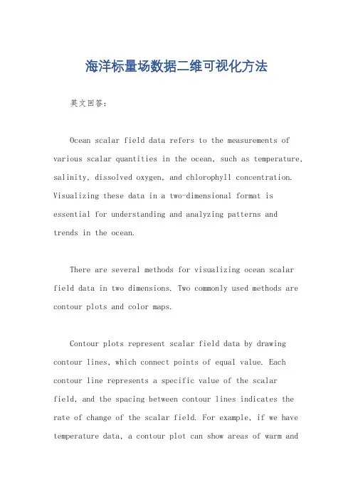
海洋标量场数据二维可视化方法英文回答:Ocean scalar field data refers to the measurements of various scalar quantities in the ocean, such as temperature, salinity, dissolved oxygen, and chlorophyll concentration. Visualizing these data in a two-dimensional format is essential for understanding and analyzing patterns and trends in the ocean.There are several methods for visualizing ocean scalar field data in two dimensions. Two commonly used methods are contour plots and color maps.Contour plots represent scalar field data by drawing contour lines, which connect points of equal value. Each contour line represents a specific value of the scalar field, and the spacing between contour lines indicates the rate of change of the scalar field. For example, if we have temperature data, a contour plot can show areas of warm andcold water and the gradients between these regions. Contour plots are useful for identifying spatial patterns and boundaries in the ocean.Color maps, on the other hand, use a color scale to represent the values of the scalar field. Each color represents a specific value, and the intensity or brightness of the color indicates the magnitude of the scalar field. For example, a color map of chlorophyll concentration can show areas of high and low productivity in the ocean. Color maps are effective for visualizing the overall distribution and variability of scalar field data.In addition to contour plots and color maps, other visualization techniques can be used to enhance the understanding of ocean scalar field data. For example, vector plots can be used to show the direction and magnitude of ocean currents by using arrows. Streamlines can be used to depict the paths of water masses orparticles in the ocean. Scatter plots can be used to explore relationships between different scalar quantities, such as temperature and salinity.Overall, the choice of visualization method depends on the specific goals and characteristics of the ocean scalar field data. It is important to select a method that effectively communicates the information and insights derived from the data. By using a combination of visualizations, scientists and researchers can gain a comprehensive understanding of the complex dynamics of the ocean.中文回答:海洋标量场数据是指海洋中各种标量量值的测量数据,例如温度、盐度、溶解氧和叶绿素浓度。
C++ Primer英文版(第5版)《C++ Primer英文版(第5版)》基本信息作者: (美)李普曼(Lippman,S.B.) (美)拉乔伊(Lajoie,J.) (美)默Moo,B.E.) 出版社:电子工业出版社ISBN:9787121200380上架时间:2013-4-23出版日期:2013 年5月开本:16开页码:964版次:5-1所属分类:计算机 > 软件与程序设计 > C++ > C++内容简介计算机书籍 这本久负盛名的C++经典教程,时隔八年之久,终迎来史无前例的重大升级。
除令全球无数程序员从中受益,甚至为之迷醉的——C++大师Stanley B. Lippman的丰富实践经验,C++标准委员会原负责人Josée Lajoie对C++标准的深入理解,以及C++先驱Barbara E. Moo在C++教学方面的真知灼见外,更是基于全新的C++11标准进行了全面而彻底的内容更新。
非常难能可贵的是,《C++ Primer英文版(第5版)》所有示例均全部采用C++11标准改写,这在经典升级版中极其罕见——充分体现了C++语言的重大进展极其全面实践。
书中丰富的教学辅助内容、醒目的知识点提示,以及精心组织的编程示范,让这本书在C++领域的权威地位更加不可动摇。
无论是初学者入门,或是中、高级程序员提升,本书均为不容置疑的首选。
目录《c++ primer英文版(第5版)》prefacechapter 1 getting started 11.1 writing a simple c++program 21.1.1 compiling and executing our program 31.2 afirstlookat input/output 51.3 awordaboutcomments 91.4 flowofcontrol 111.4.1 the whilestatement 111.4.2 the forstatement 131.4.3 readinganunknownnumberof inputs 141.4.4 the ifstatement 171.5 introducingclasses 191.5.1 the sales_itemclass 201.5.2 afirstlookatmemberfunctions 231.6 thebookstoreprogram. 24chaptersummary 26definedterms 26part i the basics 29chapter 2 variables and basic types 312.1 primitivebuilt-intypes 322.1.1 arithmetictypes 322.1.2 typeconversions 352.1.3 literals 382.2 variables 412.2.1 variabledefinitions 412.2.2 variabledeclarations anddefinitions 44 2.2.3 identifiers 462.2.4 scopeof aname 482.3 compoundtypes 502.3.1 references 502.3.2 pointers 522.3.3 understandingcompoundtypedeclarations 57 2.4 constqualifier 592.4.1 references to const 612.4.2 pointers and const 622.4.3 top-level const 632.4.4 constexprandconstantexpressions 652.5 dealingwithtypes 672.5.1 typealiases 672.5.2 the autotypespecifier 682.5.3 the decltypetypespecifier 702.6 definingourowndatastructures 722.6.1 defining the sales_datatype 722.6.2 using the sales_dataclass 742.6.3 writing our own header files 76 chaptersummary 78definedterms 78chapter 3 strings, vectors, and arrays 813.1 namespace usingdeclarations 823.2 library stringtype 843.2.1 defining and initializing strings 843.2.2 operations on strings 853.2.3 dealing with the characters in a string 90 3.3 library vectortype 963.3.1 defining and initializing vectors 973.3.2 adding elements to a vector 1003.3.3 other vectoroperations 1023.4 introducingiterators 1063.4.1 usingiterators 1063.4.2 iteratorarithmetic 1113.5 arrays 1133.5.1 definingandinitializingbuilt-inarrays 113 3.5.2 accessingtheelementsof anarray 1163.5.3 pointers andarrays 1173.5.4 c-stylecharacterstrings 1223.5.5 interfacingtooldercode 1243.6 multidimensionalarrays 125chaptersummary 131definedterms 131chapter 4 expressions 1334.1 fundamentals 1344.1.1 basicconcepts 1344.1.2 precedenceandassociativity 1364.1.3 orderofevaluation 1374.2 arithmeticoperators 1394.3 logical andrelationaloperators 1414.4 assignmentoperators 1444.5 increment anddecrementoperators 1474.6 thememberaccessoperators 1504.7 theconditionaloperator 1514.8 thebitwiseoperators 1524.9 the sizeofoperator 1564.10 commaoperator 1574.11 typeconversions 1594.11.1 thearithmeticconversions 1594.11.2 other implicitconversions 1614.11.3 explicitconversions 1624.12 operatorprecedencetable 166 chaptersummary 168definedterms 168chapter 5 statements 1715.1 simple statements 1725.2 statementscope 1745.3 conditional statements 1745.3.1 the ifstatement 1755.3.2 the switchstatement 1785.4 iterativestatements 1835.4.1 the whilestatement 1835.4.2 traditional forstatement 1855.4.3 range forstatement 1875.4.4 the do whilestatement 1895.5 jumpstatements 1905.5.1 the breakstatement 1905.5.2 the continuestatement 1915.5.3 the gotostatement 1925.6 tryblocks andexceptionhandling 1935.6.1 a throwexpression 1935.6.2 the tryblock 1945.6.3 standardexceptions 197 chaptersummary 199definedterms 199chapter 6 functions 2016.1 functionbasics 2026.1.1 localobjects 2046.1.2 functiondeclarations 2066.1.3 separatecompilation 2076.2 argumentpassing 2086.2.1 passingargumentsbyvalue 2096.2.2 passingargumentsbyreference 2106.2.3 constparametersandarguments 2126.2.4 arrayparameters 2146.2.5 main:handlingcommand-lineoptions 218 6.2.6 functionswithvaryingparameters 2206.3 return types and the returnstatement 222 6.3.1 functionswithnoreturnvalue 2236.3.2 functionsthatreturnavalue 2236.3.3 returningapointer toanarray 2286.4 overloadedfunctions 2306.4.1 overloadingandscope 2346.5 features forspecializeduses 2366.5.1 defaultarguments 2366.5.2 inline and constexprfunctions 2386.5.3 aids for debugging 2406.6 functionmatching 2426.6.1 argumenttypeconversions 2456.7 pointers tofunctions 247 chaptersummary 251definedterms 251chapter 7 classes 2537.1 definingabstractdatatypes 2547.1.1 designing the sales_dataclass 2547.1.2 defining the revised sales_dataclass 256 7.1.3 definingnonmemberclass-relatedfunctions 260 7.1.4 constructors 2627.1.5 copy,assignment, anddestruction 2677.2 accesscontrol andencapsulation 2687.2.1 friends 2697.3 additionalclassfeatures 2717.3.1 classmembersrevisited 2717.3.2 functions that return *this 2757.3.3 classtypes 2777.3.4 friendshiprevisited 2797.4 classscope 2827.4.1 namelookupandclassscope 2837.5 constructorsrevisited 2887.5.1 constructor initializerlist 2887.5.2 delegatingconstructors 2917.5.3 theroleof thedefaultconstructor 2937.5.4 implicitclass-typeconversions 2947.5.5 aggregateclasses 2987.5.6 literalclasses 2997.6 staticclassmembers 300chaptersummary 305definedterms 305contents xipart ii the c++ library 307chapter 8 the io library 3098.1 the ioclasses 3108.1.1 nocopyorassignfor ioobjects 3118.1.2 conditionstates 3128.1.3 managingtheoutputbuffer 3148.2 file input and output 3168.2.1 using file stream objects 3178.2.2 file modes 3198.3 stringstreams 3218.3.1 using an istringstream 3218.3.2 using ostringstreams 323chaptersummary 324definedterms 324chapter 9 sequential containers 3259.1 overviewof the sequentialcontainers 3269.2 containerlibraryoverview 3289.2.1 iterators 3319.2.2 containertypemembers 3329.2.3 begin and endmembers 3339.2.4 definingandinitializingacontainer 3349.2.5 assignment and swap 3379.2.6 containersizeoperations 3409.2.7 relationaloperators 3409.3 sequentialcontaineroperations 3419.3.1 addingelements toasequentialcontainer 3419.3.2 accessingelements 3469.3.3 erasingelements 3489.3.4 specialized forward_listoperations 3509.3.5 resizingacontainer 3529.3.6 containeroperationsmayinvalidateiterators 353 9.4 how a vectorgrows 3559.5 additional stringoperations 3609.5.1 other ways to construct strings 3609.5.2 other ways to change a string 3619.5.3 stringsearchoperations 3649.5.4 the comparefunctions 3669.5.5 numericconversions 3679.6 containeradaptors 368chaptersummary 372definedterms 372chapter 10 generic algorithms 37510.1 overview. 37610.2 afirstlookat thealgorithms 37810.2.1 read-onlyalgorithms 37910.2.2 algorithmsthatwritecontainerelements 380 10.2.3 algorithmsthatreordercontainerelements 383 10.3 customizingoperations 38510.3.1 passingafunctiontoanalgorithm 38610.3.2 lambdaexpressions 38710.3.3 lambdacapturesandreturns 39210.3.4 bindingarguments 39710.4 revisiting iterators 40110.4.1 insert iterators 40110.4.2 iostream iterators 40310.4.3 reverse iterators 40710.5 structureofgenericalgorithms 41010.5.1 thefive iteratorcategories 41010.5.2 algorithmparameterpatterns 41210.5.3 algorithmnamingconventions 41310.6 container-specificalgorithms 415 chaptersummary 417definedterms 417chapter 11 associative containers 41911.1 usinganassociativecontainer 42011.2 overviewof theassociativecontainers 423 11.2.1 defininganassociativecontainer 423 11.2.2 requirements onkeytype 42411.2.3 the pairtype 42611.3 operations onassociativecontainers 428 11.3.1 associativecontainer iterators 429 11.3.2 addingelements 43111.3.3 erasingelements 43411.3.4 subscripting a map 43511.3.5 accessingelements 43611.3.6 awordtransformationmap 44011.4 theunorderedcontainers 443 chaptersummary 447definedterms 447chapter 12 dynamicmemory 44912.1 dynamicmemoryandsmartpointers 45012.1.1 the shared_ptrclass 45012.1.2 managingmemorydirectly 45812.1.3 using shared_ptrs with new 46412.1.4 smartpointers andexceptions 46712.1.5 unique_ptr 47012.1.6 weak_ptr 47312.2 dynamicarrays 47612.2.1 newandarrays 47712.2.2 the allocatorclass 48112.3 usingthelibrary:atext-queryprogram 484 12.3.1 designof thequeryprogram 48512.3.2 definingthequeryprogramclasses 487 chaptersummary 491definedterms 491part iii tools for class authors 493chapter 13 copy control 49513.1 copy,assign, anddestroy 49613.1.1 thecopyconstructor 49613.1.2 thecopy-assignmentoperator 50013.1.3 thedestructor 50113.1.4 theruleofthree/five 50313.1.5 using = default 50613.1.6 preventingcopies 50713.2 copycontrol andresourcemanagement 51013.2.1 classesthatactlikevalues 51113.2.2 definingclassesthatactlikepointers 51313.3 swap 51613.4 acopy-controlexample 51913.5 classesthatmanagedynamicmemory 52413.6 movingobjects 53113.6.1 rvaluereferences 53213.6.2 moveconstructor andmoveassignment 53413.6.3 rvaluereferencesandmemberfunctions 544 chaptersummary 549definedterms 549chapter 14 overloaded operations and conversions 551 14.1 basicconcepts 55214.2 input andoutputoperators 55614.2.1 overloading the output operator [[55714.2.2 overloading the input operator ]]. 55814.3 arithmetic andrelationaloperators 56014.3.1 equalityoperators 56114.3.2 relationaloperators 56214.4 assignmentoperators 56314.5 subscriptoperator 56414.6 increment anddecrementoperators 56614.7 memberaccessoperators 56914.8 function-calloperator 57114.8.1 lambdasarefunctionobjects 57214.8.2 library-definedfunctionobjects 57414.8.3 callable objects and function 57614.9 overloading,conversions, andoperators 57914.9.1 conversionoperators 58014.9.2 avoidingambiguousconversions 58314.9.3 functionmatchingandoverloadedoperators 587 chaptersummary 590definedterms 590chapter 15 object-oriented programming 59115.1 oop:anoverview 59215.2 definingbaseandderivedclasses 59415.2.1 definingabaseclass 59415.2.2 definingaderivedclass 59615.2.3 conversions andinheritance 60115.3 virtualfunctions 60315.4 abstractbaseclasses 60815.5 accesscontrol andinheritance 61115.6 classscopeunder inheritance 61715.7 constructors andcopycontrol 62215.7.1 virtualdestructors 62215.7.2 synthesizedcopycontrol andinheritance 62315.7.3 derived-classcopy-controlmembers 62515.7.4 inheritedconstructors 62815.8 containers andinheritance 63015.8.1 writing a basketclass 63115.9 textqueriesrevisited 63415.9.1 anobject-orientedsolution 63615.9.2 the query_base and queryclasses 63915.9.3 thederivedclasses 64215.9.4 the evalfunctions 645chaptersummary 649definedterms 649chapter 16 templates and generic programming 65116.1 definingatemplate. 65216.1.1 functiontemplates 65216.1.2 classtemplates 65816.1.3 templateparameters 66816.1.4 membertemplates 67216.1.5 controlling instantiations 67516.1.6 efficiency and flexibility 67616.2 templateargumentdeduction 67816.2.1 conversions andtemplatetypeparameters 67916.2.2 function-templateexplicitarguments 68116.2.3 trailing return types and type transformation 683 16.2.4 functionpointers andargumentdeduction 68616.2.5 templateargumentdeductionandreferences 68716.2.6 understanding std::move 69016.2.7 forwarding 69216.3 overloadingandtemplates 69416.4 variadictemplates 69916.4.1 writingavariadicfunctiontemplate 70116.4.2 packexpansion 70216.4.3 forwardingparameterpacks 70416.5 template specializations 706chaptersummary 713definedterms 713part iv advanced topics 715chapter 17 specialized library facilities 71717.1 the tupletype 71817.1.1 defining and initializing tuples 71817.1.2 using a tuple toreturnmultiplevalues 72117.2 the bitsettype 72317.2.1 defining and initializing bitsets 723 17.2.2 operations on bitsets 72517.3 regularexpressions 72817.3.1 usingtheregularexpressionlibrary 729 17.3.2 thematchandregex iteratortypes 73417.3.3 usingsubexpressions 73817.3.4 using regex_replace 74117.4 randomnumbers 74517.4.1 random-numberengines anddistribution 745 17.4.2 otherkinds ofdistributions 74917.5 the iolibraryrevisited 75217.5.1 formattedinput andoutput 75317.5.2 unformattedinput/outputoperations 761 17.5.3 randomaccess toastream 763 chaptersummary 769definedterms 769chapter 18 tools for large programs 77118.1 exceptionhandling 77218.1.1 throwinganexception 77218.1.2 catchinganexception 77518.1.3 function tryblocks andconstructors 777 18.1.4 the noexceptexceptionspecification 779 18.1.5 exceptionclasshierarchies 78218.2 namespaces 78518.2.1 namespacedefinitions 78518.2.2 usingnamespacemembers 79218.2.3 classes,namespaces,andscope 79618.2.4 overloadingandnamespaces 80018.3 multiple andvirtual inheritance 80218.3.1 multiple inheritance 80318.3.2 conversions andmultiplebaseclasses 805 18.3.3 classscopeundermultiple inheritance 807 18.3.4 virtual inheritance 81018.3.5 constructors andvirtual inheritance 813 chaptersummary 816definedterms 816chapter 19 specialized tools and techniques 819 19.1 controlling memory allocation 82019.1.1 overloading new and delete 82019.1.2 placement newexpressions 82319.2 run-timetypeidentification 82519.2.1 the dynamic_castoperator 82519.2.2 the typeidoperator 82619.2.3 usingrtti 82819.2.4 the type_infoclass 83119.3 enumerations 83219.4 pointer toclassmember 83519.4.1 pointers todatamembers 83619.4.2 pointers tomemberfunctions 83819.4.3 usingmemberfunctions ascallableobjects 84119.5 nestedclasses 84319.6 union:aspace-savingclass 84719.7 localclasses 85219.8 inherentlynonportablefeatures 85419.8.1 bit-fields 85419.8.2 volatilequalifier 85619.8.3 linkage directives: extern "c" 857chaptersummary 862definedterms 862appendix a the library 865a.1 librarynames andheaders 866a.2 abrieftourof thealgorithms 870a.2.1 algorithms tofindanobject 871a.2.2 otherread-onlyalgorithms 872a.2.3 binarysearchalgorithms 873a.2.4 algorithmsthatwritecontainerelements 873a.2.5 partitioningandsortingalgorithms 875a.2.6 generalreorderingoperations 877a.2.7 permutationalgorithms 879a.2.8 setalgorithms forsortedsequences 880a.2.9 minimumandmaximumvalues 880a.2.10 numericalgorithms 881a.3 randomnumbers 882a.3.1 randomnumberdistributions 883a.3.2 randomnumberengines 884本图书信息来源:中国互动出版网。
contourplot函数Contour plot, also known as a level plot or isocontour plot, is a graphical representation of a three-dimensional surface on a two-dimensional plane. It is widely used in various scientific and engineering fields to visualize the relationship between two continuous variables, often representing a third variable through contour lines or shaded regions.In this article, we will explore the contourplot function, which is a powerful tool in data visualization. We will discuss its definition, how it works, its applications, and some examples to illustrate its usage.Definition:Contourplot is a function commonly found in data visualization libraries, such as Matplotlib in Python or ggplot2 in R. It takes in three variables, x, y, and z. The x and y variables represent the coordinates on the two-dimensional plane, while the z variable represents the value associated with each coordinate pair.The contourplot function then generates a contour plot by creating isocontour lines or shaded regions that connect points of equal z-values. These contour lines or regions help us understand the structure and behavior of the underlying surface, identifying areas of high or low values.How does it work?To generate a contour plot, the contourplot function first creates agrid of x and y values spanning the range of the data. By default, the grid is evenly spaced, but it can also be customized to manage the resolution of the plot.For each point in the grid, the contourplot function calculates the associated z-value based on the given function or dataset. It then connects points with the same z-value, producing a set of contour lines or shaded regions.The spacing between contour lines, also known as contour levels, can be customized to highlight specific regions of interest. Higher contour levels create a more detailed plot, while lower levels smooth out the plot.Applications:Contour plots are widely used in various scientific and engineering fields due to their ability to visualize complex data patterns and relationships. Some common applications include:1. Physical Sciences: Contour plots are used to represent physical phenomena such as temperature distribution, pressure gradients, and electrostatic potential. They aid in understanding the behavior of these variables in space.2. Environmental Studies: Contour plots are used to represent environmental variables such as precipitation, wind speed, and pollutant concentration. They help identify patterns and areas of interest, assisting in decision-making processes.3. Geology and Geography: Contour plots are used to represent elevation, topography, and bathymetry. They are essential tools in studying landforms, geological processes, and oceanographic features.4. Engineering and Design: Contour plots are used to represent stress distribution, heat conduction, fluid flow, and other variables in various engineering applications. They aid in optimizing designs, identifying problem areas, and visualizing simulation results.Examples:Let's explore a few examples of contourplot usage using the Matplotlib library in Python:Example 1: Temperature DistributionSuppose we have a set of temperature measurements in a two-dimensional space. We can use a contour plot to visualize the temperature distribution.```pythonimport numpy as npimport matplotlib.pyplot as plt# Generate x, y coordinatesx = np.linspace(-2, 2, 100)y = np.linspace(-2, 2, 100)X, Y = np.meshgrid(x, y)# Generate temperature valuesZ = np.sin(X) * np.cos(Y)# Create a contour plotplt.contourf(X, Y, Z, cmap='coolwarm')plt.colorbar()plt.title('Temperature Distribution')plt.xlabel('X')plt.ylabel('Y')plt.show()```In this example, we generate a grid of x and y values using`np.linspace`. We then calculate the temperature values (z-values) based on a mathematical function `Z = sin(X) * cos(Y)`. Finally, we use the `contourf` function to create a filled contour plot. We add a color bar, a title, and labels to enhance the plot's readability.Example 2: Pollutant ConcentrationSuppose we have measurements of pollutant concentrations in a two-dimensional space. We can use a contour plot to visualize the spatial distribution of pollutants.```pythonimport numpy as npimport matplotlib.pyplot as plt# Generate x, y coordinatesx = np.linspace(-5, 5, 200)y = np.linspace(-5, 5, 200)X, Y = np.meshgrid(x, y)# Generate pollutant concentration valuesZ = np.exp(-X**2 - Y**2)# Create a contour plotplt.contour(X, Y, Z, cmap='YlOrRd')plt.colorbar()plt.title('Pollutant Concentration')plt.xlabel('X')plt.ylabel('Y')plt.show()```In this example, we generate a grid of x and y values using`np.linspace`. We then calculate the pollutant concentration values (z-values) based on a mathematical function `Z = exp(-X^2 - Y^2)`. Finally, we use the `contour` function to create a contour plot. We add a color bar, a title, and labels to enhance the plot's readability.Conclusion:Contour plots are invaluable tools in data visualization, allowing us to understand complex relationships between variables in a two-dimensional space. They are widely used in various scientific and engineering fields to analyze and interpret data patterns.The contourplot function, available in data visualization libraries, enables us to generate contour plots by connecting points of equalz-values with contour lines or shaded regions. By customizing the contour levels, we can focus on specific regions of interest.Through examples, we have demonstrated how contour plots can be used to visualize temperature distributions and pollutant concentrations. With the help of the Matplotlib library in Python, we can easily generate and customize contour plots to suit our data visualization needs.In conclusion, contourplot functions are powerful tools in visualizing data relationships and patterns, and they play a vital role in understanding complex data in various scientific and engineering fields.。
matplot contourf函数解释说明1. 引言1.1 概述Matplotlib是一款功能强大的Python绘图库,广泛应用于数据可视化与科学计算领域。
其中contourf函数是Matplotlib中一个重要的绘图函数之一,用于绘制等高线图。
1.2 文章结构本文将从以下几个方面对matplot contourf函数进行深入讲解和说明:引言、Matplotlib库简介、Contour绘图原理与基本使用方法、Contourf函数进阶应用技巧以及结论与展望。
在引言部分,我们将对文章的主题和内容进行简要概述,阐明本文旨在详细介绍matplot contourf函数的相关知识和应用技巧。
1.3 目的本文旨在帮助读者全面理解Matplotlib库的重要性,并详细介绍contour绘图在数据可视化中的应用场景。
同时,通过深入讲解和实例演示contourf函数的原理、参数和用法,使读者能够掌握该函数的基本使用方法。
此外,还将介绍如何利用contourf函数进行颜色填充设置、线型修改以及标签显示方式调整等进阶技巧,并通过实例分析展示如何利用contourf函数进行二维数据可视化展示。
最后,我们将总结contourf函数的主要特点与优势,并对其未来的研究和应用方向进行展望。
通过阅读本文,读者将能够深入了解matplot contourf函数的使用方法,掌握其在数据可视化中的重要性和应用场景,并在实际项目中充分利用其功能特点进行数据可视化展示。
接下来,我们将介绍Matplotlib库的概述及其重要性。
2. Matplotlib库简介:2.1 理解Matplotlib库:Matplotlib是一个功能强大的Python绘图工具库,用于创建高质量的静态、动态和交互式可视化图形。
它是一个开源项目,被广泛应用于数据分析、科学研究以及工程领域。
Matplotlib提供了一系列函数和方法,可以轻松地绘制各种类型的图表,包括线型图、散点图、柱状图等。
matplotlib.pyplot中的contourf函数-回复Introduction:The contourf function in matplotlib.pyplot is a powerful tool for visualizing and presenting 2D scalar fields. It allows us to create filled contour plots, where each contour represents a specific value of the scalar field. In this article, we will explore the various features and uses of contourf, step by step, to understand how it can be used to effectively communicate complex data.I. Understanding Contours:To begin, it's important to understand what contours represent in a 2D plot. A contour is a line that connects points of equal value on a graph. In the case of contourf, these lines are filled to create a visual representation of the scalar field.II. Preparing the Data:Before we can use contourf, we need to have the data we want to plot. Typically, this data is in the form of a 2D grid with corresponding scalar values. For example, let's say we have adataset with temperature readings from different regions on a map. We can arrange these readings in a grid and assign corresponding temperatures to each point on the grid.III. Plotting Contours:Once we have our data prepared, we can start plotting the contours. To do this, we first import the necessary libraries, including matplotlib.pyplot. We then create a figure and an axes object using the subplots function.Next, we use the contourf function to plot the contours on the axes object. We pass in the data grid and specify the levels at which we want contours to appear. The levels parameter can be a single value, which will generate a contour at that value, or a range of values to generate multiple contours.Additionally, contourf allows us to define color maps using the cmap parameter, which determines how the colors are assigned to the different contour levels. We can choose from predefined color maps or create our own custom color maps.IV. Fine-tuning the Plot:Once the basic contours are plotted, we can enhance the visualization by adding annotations, labels, and other elements. For example, we can use the contour function to overlay line contours on top of the filled contours. We can also add a color bar to indicate the range of values represented by the colors.Moreover, contourf provides options to customize the appearance of the plot. We can adjust the line width, line color, and line style of the contours. We can also change the color and transparency of the filled areas. These options allow us to create visually appealing and informative plots.V. Advanced Features:Contourf offers advanced features to handle complex data and improve the clarity of the plot. We can use the linestyles parameter to create special contour lines, such as dashed or dotted lines, to highlight specific features. We can also control the spacing between the contour levels using the extend parameter, which enables smooth transitions between adjacent contours.Furthermore, contourf allows us to combine multiple plots in a single figure, incorporating subplots and insets. This capability is particularly useful when comparing different datasets or presenting detailed views of specific regions.VI. Applications:Contourf is widely used in a variety of fields, including meteorology, geophysics, and engineering. It can be applied to visualize weather patterns, fluid dynamics, topographic maps, and more. With its ability to effectively represent complex scalar fields, contourf helps researchers and analysts gain insights and make informed decisions based on the data.Conclusion:In summary, the contourf function in matplotlib.pyplot is a powerful tool for visualizing 2D scalar fields. With its flexible options for customizing contours, colors, and annotations, contourf enables us to create informative and visually appealingplots. By understanding the step-by-step process of using contourf, we can effectively communicate complex data and enhance our exploration of the underlying patterns and relationships.。
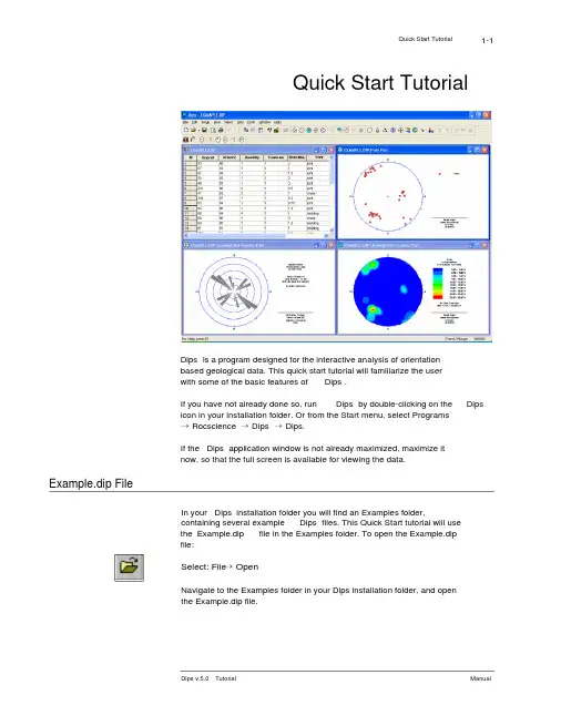
Quick Start TutorialDips is a program designed for the interactive analysis of orientationbased geological data. This quick start tutorial will familiarize the userwith some of the basic features of Dips.If you have not already done so, run Dips by double-clicking on the Dipsicon in your installation folder. Or from the Start menu, select Programs→ Rocscience → Dips → Dips.If the Dips application window is not already maximized, maximize itnow, so that the full screen is available for viewing the data.Example.dip FileIn your Dips installation folder you will find an Examples folder,containing several example Dips files. This Quick Start tutorial will usethe Example.dip file in the Examples folder. To open the Example.dipfile:Select: File → OpenNavigate to the Examples folder in your Dips installation folder, and openthe Example.dip file.You should see the spreadsheet view shown in Figure 1. A Dips file is always opened by displaying a spreadsheet view of the data. The Dips spreadsheet is also called the Grid View throughout this manual.Maximize the Grid View.Figure 1: Grid View of Example.dip file.We won’t worry about the details of this file yet, except to note that it contains 40 rows, and the following columns:?Two Orientation Columns? A Quantity Column? A Traverse Column?Three Extra ColumnsIn the next tutorial, we will discuss how to create the EXAMPLE.DIP filefrom scratch.Pole PlotCreating a Pole Plot is just one mouse click away. Select the Pole Plotoption from the toolbar or the View menu.Select: View → Pole PlotA new view displaying a Pole Plot will be generated, as shown below.Figure 2: Pole Plot of EXAMPLE.DIP data.Each pole on a Pole Plot represents an orientation data pair in the firsttwo columns of a Dips file.The Pole Plot can also display feature attribute information, based on thedata in any column of a Dips file, with the Symbolic Pole Plot option. Thisis covered later in this tutorial.ConventionAs you move the cursor around the stereonet, notice that the cursororientation coordinates are displayed in the Status Bar.The format of these orientation coordinates can be toggled with theConvention option in the Setup menu.?If the Convention is Pole Vector, the coordinates will be inTrend / Plunge format, and represent the cursor (pole) locationdirectly. This is the default setting.?If the Convention is Plane Vector, the coordinates willcorrespond to the Global Orientation Format of the currentdocument (e.g. Dip/DipDirection , Strike/DipRight ,Strike/DipLeft), and represent the PLANE corresponding to thecursor (pole) location.TIP: the quickest and most convenient way of toggling the Convention isto click on the box in the Status Bar to the left of the coordinate display,with the LEFT mouse button.The Convention also affects the format of certain data listings in Dips(e.g. the Major Planes legend, the Edit Planes and Edit Sets dialogs), andthe format of orientation data input for certain options (e.g. Add Planeand Add Set Window dialogs).NOTE: THE CONVENTION OPTION DOES NOT AFFECT THEPLOTTING OF DATA, OR THE VALUES IN THE GRID IN ANY WAY !!Poles are ALWAYS plotted using the Trend and Plunge of the pole vectorwith respect to the reference sphere, regardless of the setting of theConvention option.LegendNote that the Legend for the Pole Plot (and all stereonet plots in Dips)indicates the:?Projection Type (Equal Angle) and?Hemisphere (Lower Hemisphere).These can be changed using Stereonet Options in the Setup menu (EqualArea and Upper Hemisphere options can be used). However, for thistutorial, we will use the default projection options.Note that the Legend also indicates “61 Poles, 40 Entries”.?The EXAMPLE.DIP file has 40 rows, hence “40 entries”.?The Quantity Column in this file allows the user to recordmultiple identical data units in a single row of the file. Hence the40 data entries actually represent 61 features, hence “61 poles Let’s move on to the Scatter Plot.Scatter PlotWhile the Pole Plot illustrates orientation data, single pole symbols mayactually represent several unit measurements of similar orientation.Select the Scatter Plot option from the toolbar or the View menu, togenerate a Scatter Plot.Select: View → Scatter PlotA Scatter Plot allows the user to better view the numerical distribution ofthese measurements, since coincident pole and closely neighbouring polemeasurements are grouped together with quantities plotted symbolically.The Scatter Plot Legend indicates the number of poles represented byeach symbol.Let’s move on to the Contour Plot, which is the main tool for analyzingpole concentrations on a stereonet.Contour PlotSelect the Contour Plot option from the toolbar or the View menu, and aContour Plot will be generated.Select: View → Contour PlotFigure 3: Contour Plot of EXAMPLE.DIP data.The Contour Plot clearly shows the data concentrations. It can be seenthat there are three data clusters in the EXAMPLE.DIP file, includingone that wraps around to the opposite side of the stereonet.Since this file only contains 40 data entries, the data clustering in thiscase was apparent even on the Pole Plot. However, in larger Dips files, which may contain hundreds or even thousands of entries, cluster recognition will not necessarily be visible on Pole or Scatter Plots, and Contour Plots are necessary to identify major data concentrations. Weighted Contour PlotSince this file contains Traverse information (Traverses are discussed inthe next tutorial), a Terzaghi Weighting can be applied to Contour Plots,to correct for sampling bias introduced by data collection along Traverses.To apply the Terzaghi Weighting to the Contour Plot:Select: View → Terzaghi WeightingNote the change in the Contour Plot. Applying the Terzaghi Weightingmay reveal important data concentrations which were not apparent onthe unweighted Contour Plot. The effect of applying the TerzaghiWeighting will of course be different for each file, and will depend on thedata collected, and the traverse orientations.DO NOT USE WEIGHTED CONTOUR PLOTS FOR APPLICATIONS UNLESS YOU ARE FAMILIAR WITH THE LIMITATIONS. For adiscussion of sampling bias and the Terzaghi Weighting procedure, seethe Dips Help system.To remove the Terzaghi Weighting and restore the unweighted ContourPlot, simply re-select the Terzaghi Weighting option.Select: View → Terzaghi WeightingContour OptionsMany Contour Options are available which allow you to customize thestyle, range and number of contour intervals. We will not explore theContour Options in this tutorial, however, you are encouraged to experiment. Contour Options is available in the Setup menu, or by right-clicking on a Contour Plot.Stereonet OptionsAt this point, let’s examine the Stereonet Options dialog, which configures the basic stereonet parameters for the Contour Plot and allother stereonet plots in Dips.Right-click on the Contour Plot and select Stereonet Options, or select Stereonet Options from the Setup menu.Figure 4: Stereonet Options dialog.If you examine the Contour Plot legend, you will notice that all of the Stereonet Options are recorded here, including the Distribution method (Fisher in this case) and the Count Circle size (1% in this case) used to obtain the contours. Select Cancel to return to the Contour Plot.See the Stereonet Options topic in the Dips Help system, for complete details about all of the Dips Stereonet options.Quick Start Tutorial 1-8 Rosette PlotAnother widely used technique for representing orientations is theRosette Plot.The conventional rosette plot begins with a horizontal plane (representedby the equatorial (outer) circle of the plot). A radial histogram (with arcsegments instead of bars) is overlain on this circle, indicating the densityof planes intersecting this horizontal surface. The radial orientationlimits (azimuth) of the arc segments correspond to the range of STRIKEof the plane or group of planes being represented by the segment. Inother words, the rosette diagram is a radial histogram of strike density orfrequency.To generate a Rosette Plot, select Rosette Plot from the toolbar or theView menu.Select: View → Rosette PlotAlthough the default RosettePlot uses a horizontal baseplane, an arbitrary base planeat any orientation can bespecified in the RosetteOptions dialog. For a non-horizontal base plane, theRosette Plot represents theAPPARENT STRIKE of thelines of intersection betweenthe base plane and the planesin the Dips file.Figure 5: Rosette Plot of EXAMPLE.DIP data.Quick Start Tutorial 1-9Rosette ApplicationsThe rosette conveys less information than a full stereonet since onedimension is removed from the diagram. In cases where the planes beingconsidered form essentially two dimensional geometry (prismatic wedges,for example) the third dimension may often overcomplicate the problem.A horizontal rosette diagram may, for example, assist in blast hole designfor a vertical bench where vertical joint sets impact on fragmentation. Avertical rosette oriented perpendicular to the axis of a long topsill ortunnel may simplify wedge support design where the structure parallelsthe excavation. A vertical rosette which cuts a section through a slopeunder investigation can be used to perform quick sliding or topplinganalysis where the structure strikes parallel to the slope face.From a visualisation point of view and for conveying structural data toindividuals unfamiliar with stereographic projection, rosettes may bemore appropriate when the structural nature of the rock is simple enoughto warrant 2D treatment.Weighted Rosette PlotThe Terzaghi Weighting option can be applied to Rosette Plots as well asContour Plots, to account for sampling bias introduced by data collectionalong Traverses.?If the Terzaghi Weighting is NOT applied, the scale of the RosettePlot corresponds to the actual “number of planes” in each bin.?If the Terzaghi Weighting IS applied, the scale of the Rosette Plotcorresponds to the WEIGHTED number of planes in each bin.Do not use weighted plots for applications unless you are familiar withthe limitations. See the Dips Help system for more information.Quick Start Tutorial 1-10Adding a PlaneThe Add Plane option allows the user to graphically add a pole / plane toa stereonet plot (Pole, Scatter, Contour or Major Planes plots).First let’s switch the plot type back to a Contour Plot, since planes cannotbe added on the Rosette Plot.Select: View → Contour PlotNow select Add Plane from the toolbar or the Select menu.Select: Select → Add Plane1.Move the cursor over the Contour Plot. When the cursor isINSIDE the stereonet, an arc or “great circle” representing theplane corresponding to the cursor location (pole) will appear.Move the cursor around the stereonet, and observe the position ofthe corresponding plane.2.Note that the cursor coordinates are visible in the status bar.When the plane / pole is at a desired orientation, click the LEFTmouse button INSIDE the stereonet. (Remember that thecoordinate Convention can be toggled in the Status Bar).3.The Add Plane dialog will appear, allowing you to modify thegraphically entered orientation (if necessary), and also provideID, labeling (optional) and visibility information.For this example, enter ID = 1, Label = plane1, and leave the Visibilitycheckboxes at their default selections. Select OK.The plane / pole will be displayed on the plot, according to the visibilitysettings chosen, as shown in Figure 7.If the graphically enteredorientation is not correct, thensimply enter the correctvalues in the Add Planedialog.Figure 6: Add Plane dialog.NOTE: the visibility settings that you choose in the Add Plane dialog canbe modified AT ANY LATER TIME in the Edit Planes dialog.Quick Start Tutorial 1-11Figure 7: Added plane / pole displayed on Contour Plot.NOTE: planes created with the Add Plane option in Dips are referred toas ADDED PLANES, to distinguish them from MEAN PLANEScalculated from Sets. (Sets and mean planes are discussed in the next section).Quick Start Tutorial 1-12 Creating SetsA Set as defined in Dips, is a grouping of data created with the Add SetWindow option. The Add Set Window option allows the user to drawwindows around data clusters on a stereonet, and obtain meanorientations of data (poles) within the windows.Before we go further, note the following:?The windows created with Add Set Window are curvilinear four-sided windows, defined by two trend values and two plungevalues at opposite corners.?The windows are always formed in a CLOCKWISE direction,therefore you must always START a Set Window with one of theCOUNTER-CLOCKWISE corners.Let’s create our first Set with the small data cluster at the right side ofthe stereonet.Select: Sets → Add Set Window1.Locate the cursor at APPROXIMATELY Trend/Plunge = 55 / 65,and click the LEFT mouse button. Remember that the cursorcoordinates are displayed in the Status Bar.2.Move the mouse in a CLOCKWISE direction, and you will see acurvilinear, four-sided Set Window opening up.3.Move the cursor to APPROXIMATELY Trend/Plunge = 115 / 20,and click the LEFT mouse button. You will then see the Add SetWindow dialog.Figure 8: Add Set Window dialog.4.Don’t worry if the window coordinates are not exactly thoseshown above, as long as the window encloses the desired data.However, you may edit the coordinates at this time, if you wish.5.We will accept the default Set ID and Visibility settings, so justselect OK, and the Set will be created.Figure 9: Set Window and Unweighted mean pole / plane displayed for Set 1. Mean Plane DisplayWhen a Set is created, you will notice the following on the stereonet, asshown in Figure 9:?The Set Window will be displayed.?The mean pole / plane will be displayed according to the visibilitysettings chosen in the Add Set Window dialog. In this case, wehave displayed the Unweighted mean pole vector and plane.?Unweighted mean poles / planes are identified by an “m” beside the Set ID. Weighted mean poles / planes, if displayed, areidentified by a “w” beside the Set ID.Status Bar DisplayAfter a Set is created, the Status Bar will display the number of poles inthe Set. For this example, the Status Bar should now show:10 poles from 8 entries in Set 1The “8 entries ” refers to the number of rows of the grid within the Set. Since we have a Quantity Column in this file, each row can represent multiple data units (poles). In this case, the 8 rows actually represent 10 poles. Set Column When the FIRST Set is created, a Set Column is automatically added to the Grid. The Set Column records the Set ID of data belonging to Sets. Let ’s verify this. A Set Column is automaticallyadded to the Grid when theFIRST Set is created.A wrapped Set Window inDips automatically calculatesthe correct mean vector forSets which cross the equator. Return to the Grid View (you may select from the list of open views in the Window menu). ?Notice the Set Column, which appears AFTER the Traverse Column. ?Notice the data in the Set Column which is flagged with the Set ID = 1. These are the poles within the Set Window just created. Now return to the Contour Plot view, and we will create another Set, this time with a window which wraps around the perimeter of the stereonet. Wrapped Set Windows After you have selected the FIRST corner of a Set Window with the Add Set Window option, you will notice that if the cursor moves beyond the stereonet perimeter, it will “wrap around ” and re-appear on the opposite side of the stereonet, with the window still attached. This allows data near the perimeter, on opposite sides of the stereonet, to be selected as one Set, as illustrated in Figure 10.Figure 10: Wrapped Set Window.This useful feature of Dips automatically calculates the correct meanvector for Sets with poles plotting on opposite sides of the equator, sinceA MEAN ORIENTATION CALCULATED FROM THE LOWERHEMISPHERE ALONE WILL BE INCORRECT!!The poles within a wrapped Set window that plot on the opposite side ofthe stereonet, are incorporated into the vector addition AS NEGATIVEpoles (i.e. plunge = – plunge , trend = trend + 180), so that the mean willbe correctly calculated.Let’s create a second Set using a wrapped Set Window.Select: Sets → Add Set Window1.Locate the cursor at APPROXIMATELY Trend/Plunge = 300 / 20,and click the LEFT mouse button. Remember that the cursorcoordinates are displayed in the Status Bar.2.Move the cursor to the stereonet perimeter, and you will see thatthe Set Window reappears on the opposite side of the stereonet.3. A wrapped Set Window may seem awkward at first, but is verysimple once you get the hang of it. At worst, if you seem to “l control”, right-click the mouse and select Cancel, and start again!4.Move the cursor to APPROXIMATELY Trend/Plunge = 170 / 20,and click the LEFT mouse button. You will see the Add SetWindow dialog.5.Don’t worry if the window coordinates are not exactly thoseshown above, as long as the window encloses the desired data.However, you may edit the coordinates at this time, if you wish.6.We will accept the default Set ID (2 in this case) and Visibilitysettings, so just select OK, and the Set will be created.Figure 11: Set Windows and Unweighted mean poles / planes displayed for Sets 1 and 2.As when we created the first Set, note that the Set Window andUnweighted mean pole / plane are displayed. Also, the Status Bar shouldread (if you selected all of the poles on both sides of the stereonet):22 poles from 15 entries in Set 2Finally, note that the Set Column in the Grid View is updated to recordthe data in both Sets 1 and 2. Note that data which does NOT currentlybelong to any Set has a BLANK entry in the Set Column.Now create a third Set Window around the remaining data concentrationon the Contour Plot. (A Set Window with corners at approximately Trend/ Plunge = 190 / 40 and Trend / Plunge = 235 / 3 will do the job).Figure 12: Set Windows and Unweighted mean poles / planes displayed for Sets 1 , 2 and 3.Set InformationLet’s now look at the Info Viewer option, which provides a summary ofyour Dips file, as well as a listing of all Added Planes (Add Plane option),and all Set information.Select: File → Info ViewerFigure 13: Info Viewer display of Set information.As you scroll through the Info Viewer, you will see:?your Dips file setup information?Global mean vector orientation (i.e. the mean vector of all poles inthe file)? a list of Added Planes, if any exist (you should see the singleplane which we added earlier in this tutorial).If Sets have been created, you will then see:1. A listing of Unweighted and Weighted MEAN plane orientationsfor each Set, in both Pole Vector (Trend / Plunge) and PlaneVector format.2. A listing of Set Statistics (Fisher coefficient, and Confidence andVariability Limits at one, two and three standard deviations).3.The Set Window limits (i.e. the two corners defining each SetWindow, in Trend / Plunge format).Confidence and Variability cones can be displayed on stereonet plots, as discussed in Tutorial 3.The Info Viewer listing can be printed, copied to the clipboard, etc. The Info Viewer behaves like any other view in Dips (i.e. it can be tiled, minimized, maximized, etc.), and is automatically updated whenever new information is added to the current document (e.g. when a new Set is created). When you are finished examining the Info Viewer, close the view by selecting the × button in the upper right corner.Quick Start Tutorial 1-20Major Planes PlotThe Major Planes Plot option in Dips allows the user to view PLANESONLY on a clean stereonet, without poles or contours. In addition, alisting of plane orientations is displayed in the legend, in the formatgoverned by the current Convention (Trend / Plunge or Plane Vector).Select: View → Major PlanesThe following PLANES are displayed on a Major Planes Plot:?All ADDED planes created with the Add Plane option?All MEAN planes for Sets created with the Add Set WindowoptionFigure 14: Major Planes Plot.Only planes / poles toggled for Visibility in the Edit Planes and Edit Setsdialogs, will be displayed on the Major Planes Plot.In Figure 14 we have toggled off the display of Set Windows. This is donewith the Show Windows option in the Sets menu, which toggles thevisibility of the Set Windows on a per view basis. Let’s do that now.Select: Sets → Show WindowsMajor Planes LegendThe Major Planes legend displays the orientations of planes in the formatgoverned by the Convention (Trend / Plunge or Plane Vector). Rememberthat the Convention can be toggled at any time in the Status Bar, andwill automatically update the planes Legend. Also note:?The letter “m” beside a plane ID indicates an UNWEIGHTEDMEAN PLANE for a Set?The letter “w” beside a plane ID indicates a WEIGHTED MEANPLANE for a Set? A Plane ID with NO letter indicates an ADDED plane createdwith the Add Plane option.For our current example, we have one ADDED plane (Added Planes arealways listed first in the legend), followed by the MEAN planes for thethree Sets.Plane ColoursThe default colours used for planes in Dips are:?GREEN for all ADDED planes?RED for all MEAN planesThe user can customize ADDED plane colours in the Edit Planes dialog,and MEAN plane colours in the Edit Sets dialog. This is left as anoptional exercise. NOTE that unlike most other display options in Dips,changes to the Plane Colours (or the Plane Visibility settings) affect ALLviews for the current document, and are NOT customizable on a per viewbasis.Working with Multiple ViewsNew stereonet plot views can be generated at any time, by selecting theNew Plot View option in the Window menu. Let’s generate two new plotviews, so that we can view different plots at the same time.Select: Window → New Plot ViewBy default, a Pole Plot is always displayed when a new plot view isgenerated in this manner. Generate one more view.Select: Window → New Plot ViewNow tile the views.Select: Window → Tile VerticallyYour screen should now display:?Two Pole Plot views? A Major Planes Plot view?The Grid View.Click on one of the Pole Plot views, to make it the active view, and display a Rosette Plot.Select: View → Rosette PlotClick on the Major Planes Plot, to make it the active view, and display a Contour Plot.Select: View → Contour PlotYour screen should now look something like the following figure:Figure 15: Tiled display of four views, EXAMPLE.DIP file.We will now briefly demonstrate how display options in Dips are customizable on a per view basis.Customizing ViewsFirst we will hide the planes and Set Windows on the Pole Plot View.Show PlanesThe Show Planes option can be used to Show or Hide planes on a PER VIEW basis.Click the mouse in the Pole Plot view, to make it the active view. Now select Show Planes.Select: Select → Show PlanesNotice that ALL planes on the Pole Plot view are now hidden. However,the Set Windows are still displayed.Show WindowsTo hide the Set Windows:Select: Sets → Show WindowsThe Set Windows on the Pole Plot view are now hidden.(As an optional step, click in the Contour Plot view and select Show Windows, to re-display the Set Windows in this view).This demonstrates how planes and Set Windows can be shown or hidden on a PER VIEW basis.Display OptionsNow let’s look at the Display Options dialog. Right-click on the Pole Plot view, and select Display Options.?In the Display Options dialog, change the Stereonet colour to WHITE, and select OK.Right-click on the Rosette Plot and select Display Options.?In the Display Options dialog, change the Background colour to BLACK and change the Legend Text colour to WHITE. SelectOK.This demonstrates how colours can be customized on a PER VIEW basis.NOTE that favourite viewing options (all Display Options, Stereonet Options, and Contour Options), can be saved by the user with Auto Options in the Setup menu. Saved options can be re-applied to individual views at a later time, or saved as the program defaults, allowing the userto create their own customized version of Dips.Symbolic Pole PlotWe will now demonstrate how feature attribute analysis can be carriedout using the Symbolic Pole Plot and Chart options in Dips.First, maximize the Pole Plot view.1.Right-click on the Pole Plot and select Symbolic Pole Plot(Symbolic Pole Plot is also available in the View menu).2.In the Symbolic Pole Plot dialog, change the Plot Style toSymbolic Pole Plot.3.In the drop-down list, select the column you would like to plot.For example, select TYPE.Figure 16: Symbolic Pole Plot dialog.4.The data in the TYPE column is Qualitative, therefore we do nothave to change the Data Type (if the data were Quantitative, i.e.numeric, then we would have to select the Quantitative DataType option).5.Notice that a list of all entries in the TYPE column appears in theAllocated list area.6.Select OK, and a Symbolic Pole Plot will be generated, displayingsymbols corresponding to the entries in the TYPE column.Figure 17: Symbolic Pole Plot of data in the TYPE column.Symbolic Pole Plot LegendIn the Symbolic Pole Plot legend, you will notice a number in square brackets beside each label being plotted. This refers to the TOTALnumber of poles with that label (i.e. it accounts for the Quantity Column values). If you add the numbers in the square brackets, you will find thatthe total is equal to the number of Poles listed at the bottom of thelegend, in this case, 61.Creating a Chart from a Symbolic PlotNow let’s create a corresponding Histogram, based on our Symbolic Pole Plot.1.Right-click on the Symbolic Pole Plot and select CreateCorresponding Chart.2. A new chart view will automatically be generated, using the samedata and settings selected for the Symbolic Pole Plot.Figure 18: Histogram corresponding to Symbolic Pole Plot.The Chart can then be customized, if necessary, by right-clicking on the Chart and selecting Chart Properties (e.g. the Histogram can be converted to a Pie Chart or a Line graph).Charts can also be generated directly using the Chart option in the Select menu. The above procedure is simply a shortcut for generating a chart from an existing Symbolic Pole Plot.Query DataTo wrap up this tutorial, we will demonstrate how to quickly and easilycreate subset files from a Dips file, using the Query Data option.Select: Select → Query DataYou will see the Query Data dialog.Figure 19: Query Data dialog.Query Data allows the user to create any sort of logical expression toquery the information in any column, or any combination of columns, ofyour Dips file.Let’s first create a simple query which searches for all JOINTS with aROUGH surface, i.e.:TYPE == joint && SURFACE Includes roughQuery Example 1The first step in creating a query, is to create an Expression. As you cansee at the top of the Query Data dialog, an Expression consists of Data,Operator and Operand.1.In the Query Data dialog, click in the Data box at the left of theExpression area, and select TYPE from the drop-down list.。
Floating bar chart generated from two data sets containing minimum and maximum concentration values Read more...2D XYXY vector plot displaying Arnold's cat mapping transformation Read more...3 Point Segment Graph showing the temperature trends in four quarters. Read more...The radar chart is used primarily for data comparison. Read more...Box chart of temperature data with scatter plot and distribution overlay. Read more...Area plot of two datasets where a horizontal color gradient has been applied. Read more...Polar plot representing four dimensions: bubble size, color, direction and distance. Read more...Individual contour plots on left side ovelayed with transparency on right side. Read more...Windrose graph displaying wind speed and wind direction Read more...Ternary chart with gradient fill for layer background, and color mapping of data points using another dataset. Read morImage Graph with multiple horizontal and vertical profiles/projections. Read more...Column chart with Custom Labels Read more...Pareto chart with labels and custom colors for individual columns. Read more...Bar chart with labels Read more...Scatter plot with error bars displayed using Fill Area option. Read more...This graph shows the calculated optical density of states of a superlattice as function of the photon energy and the electriScatter plot with marginal histograms. Read more...Waterfall (or Bridge) Chart showing value changes with floating columns Read more...Fill area plot with vector overlay Read more...Two polar contour plots overlaid with one polar chart. Read more...Overlay of two contour plots. Read more...Overlay of two contour plots in one graph layer. Read more...Color-filled contour plot with color scale representing matrix data, overlaid with white contour lines representing fit matLine plot with error bars drawn in user-specified point increments. Read more...Line plot with custom tick positions and labels from data columns. Read more...Ternary plot with flexible scale Read more...Three datasets plotted as lines with error bars and semi-transparent fill areas. Read more...Stacked column plot with custom column labels. Read more...Polar scatter plot with error bars Read more...Double-Y column graph with gap across layers to avoid overlapping columns Read more...Eight-panel graph with color applied to distinguish between datasets, and symbol size adjusted to compensate for variatioSymbol plot with size and color mapped to XY data, and with transparency applied for improved visibility of overlappinTernary contour plot from worksheet with three data columns represented as ternary coordinates, and one column used toTwo-layer chart combining a histogram and a Japanese Candlestick plot to represent trading volume and open, hig five-month period. Read more...Bar graph of the African population in 2010 and 2050 (projected), grouped by gender and age. Read more...Multiple-layer figure showing the energy-level structure of the Er3+ ion in a YAG crystal. All energy levels are repre more...Contour plot with major and minor levels filled and Rainbow palette applied. Read more...Bar and scatter plot with error bars showing soil contents in Sinkiang province, China. Read more...Typical Weibull probability plot showing observed percentage on the X axis and expected cumulative percentage on theLine graph with low peaks masked. Read more...Q-Q plot using Normal distribution and the Benard Score method. Observed values are plotted on the X axis with expectScatter central plot illustrating a real-valued quadratic function. Read more...Multiiple dot chart consisting of data points plotted on a simple scale. Read more...Dot chart consisting of data points plotted on a simple scale. Read more...Multiple-Y axis plot using four curves with four different colors to depict four variables with different units. Read morePolar contour plot of semiconductor wafer thickness as a function of the radius in millimeters and the angle. Read moreMicro-Raman spectroscopy of complex nanostructured mineral systems. Read more...Cathodoluminescence (light emission stimulated by electron bombardment) of quartz expressed in a ternary plot. ReadTypical Stack Lines by Y Offsets graph with four stacked curves and an XY scaler. Read more...XYZ contour plot of 30-year mean temperature for the month of January Read more...Scatter matrix from data collected in a study of the relationship between zinc levels in soil and corn production. Read mContour plot derived from XYZ worksheet data measuring ice temperature at different depths over time. Read more...Polar plot depicting temperature distribution near the North Pole. Read more...Scatter plot depicting decay and recovery curves obtained by taking two-photon fluorescence measurements of polymer. Read more...2D graph with inset depicting plotted fit parameters and uncertainties. Read more...Contour plot showing US voters arranged on a two-dimensional policy space, with the Y-axis representing social va representing economic values (higher = more conservative). Read more...Line graphs showing the results of numerical simulation of the temporal evolution of the output power of a Tm3+:ZBL the energy level population of the Tm3+ ions. Read more...Line graphs showing results of numerical simulation of the temporal evolution of the output power of a Tm3+:ZBL inversion of the laser energy level. Read more...Line graphs showing results of numerical simulation of the temporal evolution of the output power of a Tm3+:ZBLAN fShadowgraph signals vs. scattering wave vector for a mixture of glycerol and water undergoing free diffusion in the more...Propane measurements plot employing a Log10 axis (Y) and a Reciprocal axis (X). Major and minor grid lines have be directions. Read more...Population pyramid plot comparing age and gender distribution of centenarians in different countries. Read more...This graph portrays flood impact on the morphology of channels abandoned by rivers. It uses a Contour Color Fill plot plot to show flow velocities. Read more...Bitspur graph with two panels. The top panel features a double-Y plot representing engine speed and mass air flo representing switch/control variable states over time. Read more...Box chart displaying simulated water discharge data for a water discharge station. Read more...Properties of miniature postsynaptic currents (mPSCs) at the C. elegans neuromuscular junction. This example combine into the same graph window. Read more...Histogram and probabilities chart: The histogram (bottom) provides the center, spread, and skewness of the data, while t data follows a normal distribution. Read more...Scatter plot depicting the isotope signature of N sources found in IAB iron meteorites. Read more...This geographic over/under chart represents a hypothetical investment portfolio. The graph on the left shows the por countries comprising the regions. The graph on the right shows the portfolio’s weight, minus benchmark weighting in eaCampbell diagram for checking coincidence of vibration sources with natural resonances. Read more...This two-panel graph shows an analysis of the dynamically changing shape of a single neuron over time. Read more...Contour plot depicting vertical wind velocities as a function of time and height, overlaid with a vector plot depicting winmRNA expression relative to control for two different experimental treatments, plotted as a 2D bar graph with log10 axeLine plot with log10 scale and error bars depicting the oceanic particle source flux function (orange) derived fro Environmental Aerosol Study. Read more...This custom 24-panel line and symbol graph represents the evolution of hydrochemical parameters in an aquifer which urban solid waste landfill. Read more...Scatter plot from part of a c60 buckyball study, with error bars and drop lines. Read more...Smith chart graphing impedence in transmission lines. Read more...Smith chart graphing impedence in transmission lines. Read more...Stacked histogram plots displaying the distribution of student grades per quarter. Read more...Fan performance curve for a forward curved utility blower. Read more...Two-panel line and symbol plot illustrating changes in adult cigarette smoking behavior in the United states between 196YBCO superconductor growth study using multiple sets of axes and one offset to display deposition pressure, an temperature over time. Read more...Bubble + Color Mapped Plot depicting earthquake data, both magnitude (bubble) and depth (color map). Read more...Polar plot of antenna efficiency consisting of two data plots with Origin’s Fill Area feature enabled. Read more...Floating column chart generated from two data sets containing minimum and maximum concentration values Read morStack columns and bar charts depicting statistics on the consumption of three types of rechargeable batteries. Read morAIDS vaccine research results depicted in a custom four-panel line and symbol plot. Read more...XY error bar plot showing uniformity of laminar nozzle velocity. Read more...Line and symbol plots in four panels with step connections. Read more...Vertical drop line graph with fit curve Read more...Fill area graph generated with data from a study by the Propulsion Research Center at NASA/MSFC. Read more...Area graph showing two groups of datasets plotted in separate panels. The two panels are stacked on top of one anothe more...2D waterfall and scatter plot illustrating data from experimental condensed matter physics research. Read more...Multiple panel scatter graph showing water isotope ratios for D/H, 18O/16O, and 17O/16O in and out of cirrus clouds.Water isotope ratios plotted in a 2D scatter graph. Read more...2D fill area and line plots depicting spacecraft propulsion research results. Read more...Line and symbol plots showing the results of laminar flow nozzle design. Read more...Double-Y line graph of a bubble resonance signal. Read more...Custom panel graph with line and symbol plots of spectroscopic data. Read more...Contour color fill graph of the short-time Fourier transform of Doppler data. Read more...Single-walled nanotube emission intensity plotted as a color-coded contour plot. Read more...Custom graph with Y data plotted twice - once as a column plot, and once as a scatter plot with error bars. Read more...Schild plot showing the results of a linear regression performed on raw data. The green line plots above and below bands. Read more...High-low-close plot displaying high, low, and close prices of the NASDAQ 100 stocks over a four-month period. ReadStacked histogram plots illustrating a normal distribution with a peak curve overlay. Read more...3D pie chart with an "exploded" slice. This chart was created in 3D and angled to appear 2D. Read more...Default graph generated by Origin when using the Kaplan-Meier Estimator for Survival Analysis. Read more...QC X Bar R chart used to study the fluctuation of data in a continuous process. Read more...Vector plot illustrating the effect on river water flow of two differently shaped pylons. A color graph adds magnitude as aOrigin box chart presenting data from a study of the relationship between smoking and mortality. Read more...Line and symbol graph with inset plot showing the effect of the readout temperature on the optically stimulated l (Thermalox 995). Read more...Box chart representing water discharge data over three months. Raw data is included to the left of each box in the form oMultiple-layer presentation of data from magnetic analysis of alloy powders. Read more...Four-panel graph showing the effects of varying input parameters on the objective function drain discharge in a 2D, variaScatter plot comparing a mathematical model with the actual kinematics of a pedestrian in a traffic collision. Read moreContour plot with geographical data representing the part of total solar radiation that is reflected by the Earth's surface.Scatter plot showing the absolute efficiency of an HPGe detector Read more...Four graphs with custom annotations depicting mid-range IR spectra of the acid form of zeolite SSZ-35. Read more...Multiple-lines plot depicting relative intensity data from four different measuring techniques, each represented by a diffeLine plot with cubic spline connection. Read more...Circular contour plot depicting spatial activity patterns predicted by a computational model of the visual system of a houBifurcation diagram for logistic map used in population studies under conditions of random migration. Read more...Color fill contour graph with geographical map overlay. Read more...Nine-panel graph depicting mid-range IR spectra of the acid form of zeolite SSZ-35 Read more...Line plot with inset graph depicting the anisotropic decay of 1,6-Diphenyl-1,3,5-hexatriene in toluene (25 mg/ 25 ml) atWind speed and direction over time represented in a windrose diagram. Read more...Particle analysis study represented in two-panel column/bar graph with inset plots Read more...These line plots depict the impact of hurricane Georges on a bay in South Florida. Read more...Multiple trace line graph from metal alloy analysis. Read more...The Zoom Graph plot template includes a moveable rectangle which can be used to enlarge a region of interest. Read mThese two graphs display data from a study of dislocation densities on disk-shaped semiconductor wafers. The first grap multiple worksheets. The second graph is a scatter plot of the location of a measured value on the wafer. Read more...Scatter plot displaying water column sampling locations in Massachusetts Bay, with legend showing sample details and sContour plot illustrating the influence of two different agents on the survival rate of cryopreserved red blood cells. ReadThis ternary diagram displays the packing fraction when three particle types are combined. Each line in the graph repre as a function of the fractional contribution of the three particles (course, fine, and medium) in the mixture. Read more...Hurricane weather data displayed in a stack panel graph with line plots. Read more...This graph shows a comparison between the numerical and theoretical values of spatial correlations in a Monte Carlo simThis graph displays differences between “Harmonic Oscillator” and “Morse” potential energy functions and the resultingThis multi-panel graph uses Origin’s strong layering capability to represent high-resolution electron energy-loss spectra fThis column graph presents data from a study of population trends in the United States between 1950 and 1990. Datadifferent column fill pattern. Read more...Histogram plot and normal distribution curve. A histogram plot displays the number of times a data value in a selecte more...Twenty years serving the scientific and engineering c Copyright © 2012 OriginLab Corporation. All rights reserved.Site Map | Privacy Policy | Terms of Use。
NCL online Example1.Standard subscripting设定数组v为:v = (/0,1,2,3,4,5,6,7,8,9/)则以下引用分别为:v1 = v(1:7) ; v1 contains 1,2,3,4,5,6,7 .v2 = v(1:7:3) ; v2 is an array containing the elements 1,4,7 .v3 = v(:4) ; v3 contains 0,1,2,3,4 (a missing initial integer indicates the beginning of the indices).v4 = v(8:) ; v4 contains 8,9 (a missing second index indicates the largest of the indices).v5 = v(:) ; v5 equals v (this is the same as setting v5 = v).v6 = v(2:4:-1) ; v6 contains 4,3,2 (in that order).;The algorithm is to find all numbers within the range of the firstcolon-separated pair, then step in reverse when the stride is negative.v7 = v(6) ; v7 is a scalar with value 6 .v8 = v(5:3) ; v8 contains 5,4,3 in that order (when the starting index is greater than the ending index, a reverse selection is done).v9 = v(::-1) ; v9 contains 9,8,...,0 in that order.2. Color Maps(1)用RGB值创建自己的颜色图编辑自己的颜色图,使用RGB值(Red、Green和Blue),定义一个2维的float数组,维数为n×3,第一个维数n代表颜色数(n),第二个维数代表RGB值。
Workshop 2Linear Static Analysis of a Cantilever Beam:Multiple Load CasesKeywords VersionNote: This workshop provides instructions in terms of the Abaqus Keywords interface. If you wish to use the Abaqus GUI interface instead, please see the “Interactive” version of these instructions.Please complete either the Keywords or Interactive version of this workshop.IntroductionIn this workshop you will become familiar with using load cases in a linear static analysis. You will model a cantilever beam. The left end of the beam is encastred while a series of loads are applied to the free end. Six load cases are considered: unit forces in the globalX-, Y-, and Z-directions as well as unit moments about the global X-, Y-, and Z-directions. The model is shown in Figure W2–1. You will solve the problem using a single perturbation step with six load cases and (optionally) using six perturbation steps with a single load case in each step.Figure W2–1. Cantilever beam modelW2.2 As indicated in Figure W2–1, we wish to apply forces and moments to the right end ofthe beam. However, the beam is modeled with solid C3D8I elements, which possess only displacement degrees of freedom. Thus, only forces may be directly applied to the nodes of the model. Rather than applying force couples to the model, we will apply concentrated moments to the end of the beam. To this end, all loads will be transmitted to the beam through a rigid body constraint. This approach is adopted to take advantage of the fact that the rigid body reference node possesses six degrees of freedom in three-dimensions: 3 translations and 3 rotations and thus allows direct application of concentrated moments. Rigid bodies and constraints will be discussed further inLecture 5.Defining loads and load cases in the input file1.Change to the ../abaqus_solvers/keywords/load_cases directory.2.Open the file w_beam_loadcase.inp in a text editor. The file includes all themodel data required for this problem: node, element, and set definitions; materialand section properties; and fixed boundary conditions. The history data (i.e., stepdefinition) is incomplete.plete the step definition by defining the loads and load cases. The loads willbe applied in the form of concentrated forces and moments via the *CLOAD option to the rigid body reference node. This node is contained in node set refPt. Forexample, for the force acting along the axial direction of the beam (i.e., the X-direction), the following load case may be defined:*Load Case, name=Force-X*CloadrefPt, 1, 1.0*End Load Case4.The complete step definition should resemble the following:*Step, name=BeamLoadCases, perturbation*Static***Load Case, name=Force-X*CloadrefPt, 1, 1.0*End Load Case***Load Case, name=Force-Y*CloadrefPt, 2, 1.0*End Load Case***Load Case, name=Force-Z*CloadrefPt, 3, 1.0*End Load Case***Load Case, name=Moment-X*CloadrefPt, 4, 1.0*End Load Case***Load Case, name=Moment-Y*CloadrefPt, 5, 1.0*End Load Case***Load Case, name=Moment-Z*CloadrefPt, 6, 1.0*End Load Case***End StepNote that the fixed-end boundary conditions have been defined as part of the model data, and as such, are active in each load case.5.Save the input file.6.Submit the job for analysis by entering the following command at your systemprompt:abaqus job=w_beam_loadcase7.Monitor the status of the job by looking at the log (.log) or status (.sta) files.Viewing the analysis results1.When the job has completed successfully, start a session of Abaqus/Viewer byentering the following command at your system prompt:abaqus viewer odb=w_beam_loadcaseAbaqus/Viewer opens the output database file w_beam_loadcase.odb created by the job and displays the undeformed model shape. Examine the results of the analysis. Note that load case output is stored in separate frames in the outputdatabase file. Use the Frame Selector (click in the context bar) to choosewhich load case is displayed (alternatively, open the Step/Frame dialog box byselecting Result→Step/Frame). Figure W2–2, for example, shows contour plots of the Mises stress for each of the load cases.Force-X Force-Y Force-ZMoment-X Moment-Y Moment-ZFigure W2–2. Mises stress contoursCombining results from the load cases and envelope plotsYou will now linearly combine the results of each load case to plot the stress and deformation in the beam under a given load combination. Recall that each load case is based on a unit load; the results of each load case will be scaled relative to those obtained for LC-Force-Y when combining the data.1.From the main menu bar, select Tools→Create Field Output→From Frames.2.In the dialog box that appears, accept Sum values over all frames as theoperation.3.In the Frames tabbed page, click . In the Add Frames dialog box thatappears, choose Step-1 as the step from which to obtain the data. Click Select All and then click OK to close the dialog box.4.Remove the initial frame; for the remaining frames, enter the scale factors shownin Figure W2–3.Figure W2–3 Scale factors for linear combination of load cases.5.Switch to the Fields tabbed page to examine the data that will be combined.Accept the default selection (all available field data) and click OK to close thedialog box.6.From the main menu bar, select Result→Step/Frame.W2.6 7.In the Step/Frame dialog box, select Session Step as the active step for outputand click OK.8.Plot the Mises stress as shown in Figure W2–4. Note that this figure has beencustomized to overlay the undeformed model shape on the contour plot and adeformation scale factor of 5e4 has been used.Figure W2–4 Mises stress due to combined loading.9.Now create an envelope plot of the maximum stress in the beam:a.From the main menu bar, select Tools→Create Field Output→FromFrames.b.In the dialog box that appears, select Find the maximum value over allframes as the operation.c.In the Frames tabbed page, click . In the Add Frames dialog boxthat appears, choose Step-1 as the step from which to obtain the data.Select all but the initial frame then click OK to close the dialog box.d.Switch to the Fields tabbed page. Unselect all output and then select onlyS and U.e.Click OK to close the dialog box.f.From the main menu bar, select Result→Step/Frame.g.In the Step/Frame dialog box, select Session Step as the active step foroutput and The maxmum value over all selected frames as the frame,as shown in Figure W2–5.W2.7Figure W2–5 Frame selection for envelope plot.h.In the Field Output dialog box (Result→Field Output), select S_max asthe primary variable and U_max as the deformed variable.i.Plot the Mises stress as shown in Figure W2–6. Note that this figure hasbeen customized to overlay the undeformed model shape on the contourplot and a deformation scale factor of 5e4 has been used.Figure W2–6 Envelope plot of maximum Mises stress.Using Multiple Perturbation Steps (Optional)Now perform the same analysis using multiple perturbation steps rather than multiple load cases.1.Open the file w_beam_multstep.inp in a text editor. As before, the fileincludes all the model data required for this problem: node, element, and setdefinitions; material and section properties; and fixed boundary conditions. Thehistory data (i.e., step definition) is incomplete.plete the history data by defining the steps. As before, the loads will beapplied in the form of concentrated forces and moments via the *CLOAD option tothe rigid body reference node. This node is contained in node set refPt. ForW2.8 example, for the force acting along the axial direction of the beam (i.e., the X-direction), the following step may be defined:*Step, name=Force-X, perturbation*Static*CloadrefPt, 1, 1.*End Step3.The complete set of step definitions should resemble the following:*Step, name=Force-X, perturbation*Static*CloadrefPt, 1, 1.0*End Step***Step, name=Force-Y, perturbation*Static*CloadrefPt, 2, 1.0*End Step***Step, name=Force-Z, perturbation*Static*CloadrefPt, 3, 1.0*End Step***Step, name=Moment-X, perturbation*Static*CloadrefPt, 4, 1.0*End Step***Step, name=Moment-Y, perturbation*Static*CloadrefPt, 5, 1.0*End Step***Step, name=Moment-Z, perturbation*Static*CloadrefPt, 6, 1.0*End StepNote that the fixed-end boundary conditions have been defined as part of themodel data, and as such, are active in each step.4.Save the input file.5.Submit the job for analysis by entering the following command at your systemprompt:abaqus job=w_beam_multstep6.Monitor the status of the job by looking at the log (.log) or status (.sta) files.7.When the job has completed successfully, open the output databasew_beam_multstep.odb created by the job in Abaqus/Viewer and compare theresults obtained using both modeling approaches. You will find that the results are identical.Comparing solution timesNext, open the message (.msg) file for each job in the job monitor. Scroll to the bottom of the file and compare the solution times. You will notice that the multiple step analysis required 2.5 times as much CPU time as the multiple load case analysis. For a small model such as this one, the overall analysis time is small so speeding up the analysis by a factor of three may not appear significant. However, it is clear that for large jobs, the speedup offered by multiple load cases will play a significant role in reducing the time required to obtain a solution for a given problem.Multiple load case analysis:ANALYSIS SUMMARY:TOTAL OF 1 INCREMENTS0 CUTBACKS IN AUTOMATIC INCREMENTATION1 ITERATIONS1 PASSES THROUGH THE EQUATION SOLVER OF WHICH::THE SPARSE SOLVER HAS BEEN USED FOR THIS ANALYSIS.JOB TIME SUMMARYUSER TIME (SEC) = 0.10000SYSTEM TIME (SEC) = 0.10000TOTAL CPU TIME (SEC) = 0.20000WALLCLOCK TIME (SEC) = 1Multiple perturbation step analysis:ANALYSIS SUMMARY:TOTAL OF 6 INCREMENTS0 CUTBACKS IN AUTOMATIC INCREMENTATION6 ITERATIONS6 PASSES THROUGH THE EQUATION SOLVER OF WHICH::THE SPARSE SOLVER HAS BEEN USED FOR THIS ANALYSIS.JOB TIME SUMMARYUSER TIME (SEC) = 0.5000SYSTEM TIME (SEC) = 0.2000TOTAL CPU TIME (SEC) = 0.7000WALLCLOCK TIME (SEC) = 2Note: Complete input files are available for your convenience. You may consult these files if you encounter difficulties following the instructions outlined here or if you wish to check your work. The input files are named w_beam_loadcase_complete.inpw_beam_multstep_complete.inpand are available using the Abaqus fetch utility.。
Exmaple5——contour plots over maps这个示例从netCDF文件中读取数据,并且展示如何命名维度。
如何获得现有的颜色图并且改变它的值,如何在各种地图投影上叠加等值线图,如何填充特定的等值线,如何掩蔽,如何在你任意想要的位置绘制文本字符串。
这个示例从netCDF文件中读取数据并且在不同的地图投影上创建了4个等值线图。
从等值线和地图两个方面改变了resources。
运行这个示例,必须下载以下文件:gsun05n.ncl,然后键入:nclgsun05n.ncl示例5代码及解释1. load "$NCARG_ROOT/lib/ncarg/nclscripts/csm/gsn_code.ncl"2.3. begin4.data_dir = ncargpath("data") ; Get ready to open three netCDF files.5.cdf_file1 = addfile(data_dir + "/cdf/941110_P.cdf","r")6.cdf_file2 = addfile(data_dir + "/cdf/sstdata_netcdf.nc","r")7.cdf_file3 = addfile(data_dir + "/cdf/Pstorm.cdf","r")打开三个netCDF文件,cdf_file1、cdf_file2和cdf_file3是在addfile函数中指定的三个文件。
8.9.psl = cdf_file1->Psl ; Store some data from the three netCDF10.sst = cdf_file2->sst ; files to local variables.11.pf = cdf_file3->p从刚刚打开的三个netCDF中读取一些数据,并且将它们存储在本地的NCL变量中。
psl是一个在纬度/经度格点测量的压力值的2维数组,sst是一个在纬度/经度和12个不同时间步长上测量的海洋表面温度的3维数组。
pf是在纬度/经度格点和64个不同时间步长上测量的压力值的3维数组。
请注意:本地NCL变量和netCDF文件变量中所使用的不同的变量名字(如,pf和cdf_file->p)。
这是可以选择的,此示例中是为了展示你可以给你想要命名的变量随意命名。
12.13.psl@nlon = dimsizes(psl&lon) ; Store the sizes of the lat/lon14.psl@nlat = dimsizes(psl&lat) ; arrays as attributes of the psl15.pf@nlon = dimsizes(pf&lon) ; and pf variables.16.pf@nlat = dimsizes(pf&lat)Psl和pf都包含叫做“lat”和“lon”的坐标变量,因此获得这些属性变量的常量并且把它们的值以psf和pf的属性存储起来。
17.18.sst!1 = "lat" ; Name dimensions 0 and 1 of sst19.sst!2 = "lon" ; "lat" and "lon.20.sst&lat = cdf_file2->lat ; Create coordinate variables21.sst&lon = cdf_file2->lon ; for sst and store the sizes22.sst@nlon = dimsizes(sst&lon) ; of the arrays as attributes23.sst@nlat = dimsizes(sst&lat) ; of sst.sst唯一的坐标变量是“time”,和它的第一个维度相对应(这是在先前的文件中事先确定的)。
使用iscoord函数来确定变量是否含有该特定的坐标变量。
在18-21行中,因为sst只有第一个维度是命名过的,你可以给sst创建named dimensions和叫做“lat”和“lon”的第二个、第三个坐标变量。
在22-23行,存储lat和lon数组的长度作为sst变量。
请记住:为了创建另一个变量的坐标变量,它必须与变量的一个named dimension有相同的名字。
24.25.wks = gsn_open_wks("x11","gsun05n") ; Open a workstation.26.27. ;----------- Begin first plot -----------------------------------------在地理图上绘制等值线图。
28.29.resources = True30.31.resources@sfXCStartV = min(psl&lon) ; Define where contour plot32.resources@sfXCEndV= max(psl&lon) ; should lie on the map plot.33.resources@sfYCStartV = min(psl&lat)34.resources@sfYCEndV= max(psl&lat)为了在一个地图上重复显示任何图,必须在地图上指定你想要显示地图的经度和纬度值。
这是通过在重复显示的图上的经度坐标指定X轴坐标,在纬度坐标指定Y轴坐标来完成的。
对于一个等值线图,如果你的网格是等间距分布的,那么你可以使用ScalarField resources sfXCStartV和sfXCEndV来设定X轴的最小值和最大值,使用sfYCStartV和sfYCEndV来设定Y轴的最小值和最大值。
如果你有等间距分布的数组值来表示坐标轴,那么你可以使用sfXArray和sfYArray resources来设置数组值。
如果你的网格不是等间距分布的,你必须使用在example 2示例2中描述的sfXArray和sfYArray来确定坐标轴的范围。
在这个示例中,使用*StartV和*EndV resources来确定纬度、经度坐标轴的最小值和最大值。
因为psl&lat和psl&lon是psl的坐标变量,这就意味着它们代表了测量psl 的维度值和经度值。
因此,使用这些坐标变量莱维重复显示的等值线图提供经度/维度值的最小值和最大值。
min和max函数能够提取任何维度的数组并且返回该数组的最小值和最大值。
请注意:如果你没有为确定X和Y轴的最小值和最大值设定任何的ScalarField resources,那么最小值的默认值是0.0,最大值的默认值分别是n-1和m-1,n是psl在X方向上的点的个数,m是psl在Y方向上的点的个数。
这将导致等值线图会在纬度/经度(0.,0.,)和(m-1,n-1)角落显示,而并没有任何意义。
35.36.map = gsn_contour_map(wks,psl,resources) ; Draw contours over a map.在地图上创建并且绘制psl变量的等值线图。
默认的地图投影是圆柱等距投影。
gsn_contour_map函数的第一个参数是对于前一个调用gsn_open_wks的返回的工作站变量。
接下来的参数是将要绘制的2维标量场,可以是float、double或者integer类型。
最后的参数是逻辑值,表明是否设置了任何的resources。
请注意:等值线图覆盖了整张梯度。
这是因为在31-34行中指定的纬度值是从-90~90,经度值是从-180~180(可以通过使用print来将这些值打印出来而验证)。
非常重要,请注意:gsn_contour_map函数实际上是创建了两个图,等值线图和地图。
地图是从函数返回的,等值线图是作为叫做“contour”地图的一个变量返回的。
当你在一个图上覆盖另外一个图时,被覆盖的图叫做“基图”,覆盖在基图上的图叫做“覆盖图”。
函数gsn_*创建这些覆盖图通常以函数值范围基图,同时覆盖图通常是基图的属性。
当你使用setvalues语句来改变resourcees时,这些信息变得非常有用,见example 9示例9。
37.38. ;----------- Begin second plot -----------------------------------------在正投影上绘制sst(海洋表面温度)第一个时间步长的等值线图,并且为以stipple类型来填充等值线、隐蔽陆地上的等值线使等值线图显得稍大来设置一些resources。
介绍一些等值线绘制顺序和地图组件的概念(这是为了使你得到想要的隐蔽的效果)。
39.40.getvalues wks ; Retrieve the default color map.41."wkColorMap" : cmap42.end getvalues使用getvalues获得使用的默认的颜色图并且将它存储在当地变量中(在该例中是cmap,但是你可以随意称呼该变量)。
颜色图和你用gsn_open_wks中调用而打开的工作站是相联系的,因此它是“Workstation”resources组中的一部分,以“wk”开头。
default color map默认的颜色图有32个条目(每个条目都是RGB值),所以NCL为cmap分配了一个32×3的float数组。
在示例4example 4中更加详细的描述了getvalues语句。
43.44.cmap(0,:) = (/1.,1.,1./) ; Change background to white.45.cmap(1,:) = (/0.,0.,0./) ; and foreground to black.46.gsn_define_colormap(wks, cmap)颜色index0和1分别代表了背景色和前景色,在默认情况下,背景色是黑色而前景色是白色。
使用刚刚获得的颜色图(cmap),将背景色设为白色,前景色设为黑色。
用RGB值来设置颜色,白色用(1.,1.,1.)表示、黑色用(0.,0.,0.)表示。