A Boundary Condition for Simulation of Flow over Porous Surfaces,” AIAA 20012412
- 格式:pdf
- 大小:993.64 KB
- 文档页数:13
附面层抽吸位置对翼型绕流分离控制的影响张旺龙;谭俊杰;陈志华;任登凤【摘要】为了深入研究抽吸作用位置对翼型绕流分离控制效果的影响,采用HLLC 格式和双时间步长LU-SGS隐式算法对二维可压N-S方程进行数值求解,数值模拟了雷诺数Re为6 000时,NACA0012翼型在上翼面抽吸控制下的翼型绕流流场.研究了抽吸区域位置对翼型流动分离和翼型气动性能的影响.结果表明:同一抽吸系数下,合理的抽吸位置是有效改善翼型气动性能的重要因素,并且不同抽吸位置的作用机制不同.对于以开式分离为特征的NACA0012翼型绕流,其合理抽吸区域位于翼型前缘分离区内.【期刊名称】《南京理工大学学报(自然科学版)》【年(卷),期】2013(037)005【总页数】6页(P710-715)【关键词】附面层;抽吸位置;翼型绕流;分离控制【作者】张旺龙;谭俊杰;陈志华;任登凤【作者单位】南京理工大学能源与动力工程学院,江苏南京210094;南京理工大学能源与动力工程学院,江苏南京210094;南京理工大学瞬态物理国家重点实验室,江苏南京210094;南京理工大学能源与动力工程学院,江苏南京210094【正文语种】中文【中图分类】V211.3低雷诺数下的绕翼型非定常流动研究在飞行器设计中有着重要作用[1]。
随着高空无人飞行器和微型飞行器的不断发展,高空低雷诺数条件下高升阻比翼型的气动设计问题日益凸显,深入研究并控制翼型在低雷诺数条件下广泛存在的层流附面层分离现象,是提高低雷诺数下飞行器性能的迫切需要。
在低雷诺数条件下,翼型绕流常常处于层流状态,其抵抗逆压梯度的能力较弱,容易产生分离等非定常现象,对翼型的升阻力等气动性能产生严重的影响。
针对这种情况,人们一直在寻求有效控制流动的方法,试图通过改变飞行器边界层的流动结构,以达到消涡、减阻和提高推进效率及飞行稳定性的目的。
而在翼型吸力面开孔形成缝隙多孔表面,通过抽吸方式吸除一部分低能流体,延迟逆压梯度发生,减小壁面处速度剖面的曲率,可以达到抑制边界层分离[2],减少流动损失,实现对翼型流动控制的目的。
abaqus接触分析abaqus—接触分析(转)已有 264 次阅读2010-8-24 19:39 |1、塑性材料和接触面上都不能用C3D20R和C3D20单元,这可能是你收敛问题的主要原因。
如果需要得到应力,可以使用C3D8I (在所关心的部位要让单元角度尽量接近90度),如果只关心应变和位移,可以使用C3D8R, 几何形状复杂时,可以使用C3D10M。
2、接触对中的slave surface应该是材料较软,网格较细的面。
3、接触面之间有微小的距离,定义接触时要设定“Adjust=位置误差限度”,此误差限度要大于接触面之间的距离,否则ABAQUS会认为两个面没有接触:*Contact Pair, interaction="SOIL PILE SIDE CONTACT", small sliding,adjust=0.2.4、定义tie时也应该设定类似的position tolerance: *Tie,name=ShaftBottom, adjust=yes, position tolerance=0.15、 msg文件中出现zero pivot说明ABAQUS无法自动解决过约束问题,例如在桩底部的最外一圈节点上即定义了tie,又定义了contact, 出现过约束。
解决方法是在选择tie或contact的slave surface时,将类型设为node region, 然后选择区域时不要包含这一圈节点(我附上的文件中没有做这样的修改)。
6、接触定义在哪个分析步取决于你模型的实际物理背景,如果从一开始两个面就是相接触的,就定义在initial或你的第一个分析步中;如果是后来才开始接触的,就定义在后面的分析步中。
边界条件也是这样。
7、我在前面上传的文件里用*CONTROL设了允许的迭代次数18,意思是18次迭代不收敛时,才减小时间增量步(ABAQUS默认的值是12)。
一般情况下不必设置此参数,如果在msg文件中看到opening和closure的数目不断减小(即迭代的趋势是收敛的),但12次迭代仍不足以完全达到收敛,就可以用*CONTROL来增大允许的迭代次数。
钢质固定平台,是目前海上油(气)生产中应用最多的一种结构形式。
钢质固定平台中最多的是导管架式平台,主要由三大部分组成:导管架、桩和甲板组块[1]。
导管架式平台一般都是在陆地进行建造然后再装船拖运到海上安装。
装船方式有直接吊装上船、小车装船(Self-Propelled Modular Transporter,SPMT)和拖拉滑移上船三种方式[2]。
采用直接吊装上船法,一般甲板都是直立建造的,并在其顶部设置有吊点。
该方式在施工前要求平台建造方位与运输驳船靠码头时的方位协调一致,尽量减少起吊过程中浮吊的旋转,同时受吊装用驳船浮吊实际吊装能力限制[3]。
小车装船需考虑小车分组设计,而对于小车分组及布置问题,还没有详细的理论作为设计基础[4],且目前工程上应用小车装船的主要是1000t左右的小型模块。
在工程实际应用中考虑到场地实际情况、平台的总重相对较大以及吊装用驳船浮吊实际吊装能力,结合经济成本,大部分平台均需采用拖拉滑移方式上船[5]。
由于平台拖拉滑移上船是一个过程,在此过程中要考虑到各种情况的出现,到目前为止关于平台拖拉滑移上船工况边界条件的模拟还没有一个统一的做法。
本文以四腿四桩甲板组块滑移装船为例,分别采用工程实际应用中较为普遍的3种方式模拟边界条件,并对计算结果加以对比,得出一些具有指导意义的建议。
1 边界条件模拟方法分析由美国Bentley公司开发研制的SACS(Structural Analysis Computer System)软件专门用于海洋结构工程的静动力结构分析[6],目前国内外导管架式平台普遍采用该软件进行结构设计。
海洋平台组块码头滑移装船过程,是海洋工程施工作业过程中一个非常关键的组成部分,一旦出现事故,将造成无法估量的损失。
海洋平台上部组块的滑移装船工况计算是组块安装作业中的一个临时工况,在用SACS软件对该工况受力情况进行模拟时,边界条件一般采用设置GAP单元的形式。
组块的滑移装船主要是在码头驳船上的线性绞车牵引下组块连同滑靴一起滑移到驳船上事先设置好的滑道上,再由驳船将其运送到指定海域与导管架进行组对。
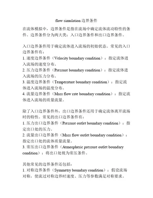
flow simulation边界条件在流体模拟中,边界条件是指在流场中确定流体流动特性的条件。
边界条件分为两大类:入口边界条件和出口边界条件。
入口边界条件用于确定流体进入流场的初始状态。
常见的入口边界条件有:1. 速度边界条件(Velocity boundary condition):指定流体进入流场的速度分布。
2. 压力边界条件(Pressure boundary condition):指定流体进入流场的压力分布。
3. 温度边界条件(Temperature boundary condition):指定流体进入流场的温度分布。
4. 流量边界条件(Mass flow rate boundary condition):指定流体进入流场的质量流量。
除了入口边界条件外,出口边界条件还用于确定流体离开流场时的特性。
常见的出口边界条件有:1. 压力出口边界条件(Pressure outlet boundary condition):指定出口处的压力。
2. 流量出口边界条件(Mass flow outlet boundary condition):指定出口处的流体质量流量。
3. 常压出口边界条件(Atmospheric pressure outlet boundary condition):将出口处视为常压条件。
其他常见的边界条件还包括:1. 对称边界条件(Symmetry boundary condition):假设流场对称,使流过对称边界时速度、压力等参数满足对称要求。
2. 壁面边界条件(Wall boundary condition):指定流场与固体墙壁接触时的流动状态,通常要考虑壁面摩擦对流体的影响。
3. 切向旋转平均边界条件(Tangential average boundary condition):常用于旋转机械中,用于对流场的切向部分进行平均处理。
4. 界面边界条件(Interface boundary condition):用于模拟不同相流体之间的界面,常用于多相流动模拟中。
使用AnsysFluent进行流体力学仿真教程Chapter 1: Introduction to ANSYS FluentIn this chapter, we will provide an overview of ANSYS Fluent and explain its importance in the field of fluid dynamics simulation. ANSYS Fluent is a powerful computational fluid dynamics (CFD) software used for simulating and analyzing fluid flows. It enables engineers and scientists to study the behavior of fluids, predict their performance in various scenarios, and optimize the design of systems involving fluid flow.Chapter 2: Pre-ProcessingThe pre-processing stage involves preparing the geometry of the system and defining the desired fluid flow conditions. ANSYS Fluent provides a variety of tools to import and manipulate geometry files, such as creating boundaries, defining initial conditions, and specifying material properties. Additionally, it allows users to create a mesh grid that discretizes the computational domain into smaller elements for accurate simulations.Chapter 3: Boundary ConditionsBoundary conditions play a crucial role in defining the behavior of the fluid flow simulation. In this chapter, we will explain the different types of boundary conditions available in ANSYS Fluent, including velocity inlet, pressure outlet, wall, and symmetry. Each boundarycondition has specific input parameters that need to be defined, such as velocity magnitude, pressure, and temperature.Chapter 4: Solver SettingsThe solver settings determine the numerical methods used to solve the fluid flow equations in ANSYS Fluent. This chapter will introduce the various solver options available, including pressure-based and density-based solvers. It will also discuss the importance of convergence criteria and the influence of physical properties, such as turbulence models and turbulence intensity.Chapter 5: Post-ProcessingOnce the simulation is complete, post-processing is performed to analyze and visualize the results. In ANSYS Fluent, users have access to a range of post-processing tools, such as contour plots, vector plots, velocity profiles, and pressure distribution. This chapter will explain how to interpret these results to gain insights into the fluid flow behavior and make informed design decisions.Chapter 6: Advanced FeaturesIn this chapter, we will explore some of the advanced features of ANSYS Fluent that can enhance the accuracy and efficiency of fluid flow simulations. These include multiphase flow simulations, combustion modeling, heat transfer analysis, and turbulence modeling. We will provide step-by-step instructions on how to set up and run simulations using these advanced features.Chapter 7: Case StudiesTo further illustrate the capabilities of ANSYS Fluent, this chapter will present a series of case studies involving different fluid flow scenarios. These case studies will cover a range of applications, such as fluid flow in pipes, aerodynamics of a car, and natural convection in a room. Each case study will include the problem statement, simulation setup, and analysis of the results.Chapter 8: Troubleshooting and TipsANYS Fluent, like any software, can sometimes encounter issues or produce unexpected results. In this chapter, we will discuss common troubleshooting techniques and provide tips for optimizing simulation setup and improving simulation accuracy. This will include techniques for mesh refinement, convergence improvement, and understanding error messages.Conclusion:ANSYS Fluent is a powerful tool for conducting fluid dynamics simulations. In this tutorial, we have covered the fundamental aspectsof using ANSYS Fluent, including pre-processing, boundary conditions, solver settings, post-processing, advanced features, and troubleshooting. By following this tutorial, users can gain a solid foundation in conducting fluid flow simulations using ANSYS Fluent and leverageits capabilities to analyze and optimize fluid flow systems in various applications.。
Defining object boundary conditionsBoundary conditions are specified and enforced at nodes in the finite element mesh. The basic procedure for setting any boundary condition except Contact is the same:1.Select the appropriate condition type.2.Select the direction (where applicable).3.Select the nodes to which boundary conditions will be applied usingone of the selection tools in the lower left button bar.4.Apply the boundary conditions.The selected nodes will be highlighted. To apply the boundary conditions click the Generate BCC's button. Colored markers will highlight the nodes to which boundary conditions have been applied. To delete specific boundary conditions, select the start and end nodes, and click the Delete BCC's button. To delete all boundary conditions of the specified type and direction, click the Initialize BCC's button.Note : You can either select faces of the surface by using the surface patches feature or use the node button to select individual nodes.Deformation boundary conditionsVelocityVelocity of each node can be specified independently in the x and y directions (or x, y, and z directions in 3d). Velocity boundary conditions are normally set to zero for symmetry conditions (see section on symmetry in this manual), but may also be set to a specified non-zero value for processes such as drawing in which a workpiece is pulled through a die.ForceForce boundary conditions specify the force applied to the node by an external object. The force is specified in default units. For die stress analysis, the force that the die exerted on the workpiece can be reversed and interpolated onto the dies by using the interpolation function. Refer to the tutorial labs on die stress analysis for a detailed procedure for using force interpolation to perform die stress analysis.PressureThe pressure boundary conditions specifies a uniform, or linearly varying, force per unit area on the element faces connecting the specified nodes. Displacement and shrink fitA specified displacement can be specified in any direction for each node. This is frequently used for specifying shrink fit conditions between a die insert and a shrink ring. More information on this is available in the section on die stress analysis in this manual.MovementThe movement of nodes on an object can be specified. If the movement boundary condition is specified, object movement controls must also be specified.ContactThe Contact boundary condition displays interobject boundary contact conditions on a given object. The user should gain some experience with DEFORM before using this option. The contact conditions are stored in three components to represent the fact that there are three degrees of freedom for any given node.ThermalHeat exchange with the environmentThis boundary condition specifies that heat exchange between element faces bounded by these nodes and their environment should occur. The contact boundary condition determines whether exchange will occur to the ambient atmosphere or to a contacting object.Heat fluxSpecifies an energy flux per unit area over the face of the element bounded by the nodes. Units are energy/time/area.Nodal heatSpecifies a heat source at the given nodes. Units are energy/time. TemperatureSpecifies a fixed temperature at the given nodes.Heat Exchange windowsThis function allows the user to define heat exchange conditions for local areas on a body by use of three dimensional window. To use heat exchange windows, perform the following actions:1.Go to the Boundary Conditions window.2.Select the Thermal tab.3.Select the Heat exchange windows button.4.Note the tools in the lower left corner of the display windowchanges and the new heat exchange window that comes up.5.At this point, heat exchange windows can be defined using the toolsin the lower left corner of the display window. Each window has its ownlocal environmental temperature, convection coefficient and emissivity.See Figure for an example heat exchange window.6.You can define up to 20 independent windows by the method. If tworegions share the same space, the lower number window wins. Diffusion [DIF]Diffusion with the environmentSpecifies diffusion of the dominant atom through the boundary elements bordered by the indicated nodes. Environment dominant atom content and surface reaction rate are specified under the Simulation Controls, Processing Conditions menu. Environment content and reaction rate for various regions of the part may be modified by using diffusion windows.Fixed atom contentSpecifies a fixed dominant atom content at the given nodes.Atom fluxSpecifies a fixed dominant atom flux rate over the elements bordered by the indicated nodes.2.4.11. Contact boundary conditionsContact boundary conditions are applied to nodes of a slave object, and specify contact between those nodes and the surface of a master object (see master-slave relationships under the Interobject data section). If a node is specified to be in contact with a particular object, it will placed on the surface of that object. If this requires changing the position of that node, it will be changed as necessary. Contact boundary conditions are generated under the InterObject , Contact Boundary Conditions.It is for this reason that the user should be VERY careful with how contact is specified. If it is improperly used, the mesh may be damaged and very often remeshing cannot aid this situation since the AMG cannot interpret the users intentions.Contact boundary conditions can be displayed for a given object using the Objects, Boundary Conditions, Advanced Deformation BCC's icon.。

comsol多物理场耦合仿真流程英文回答:The simulation process for coupling multiple physics fields in COMSOL involves several steps. First, you need to define the geometry of your model. This includes specifying the dimensions and shape of the objects in your simulation. Once the geometry is defined, you can assign the appropriate material properties to each object. This step is crucial as it determines how each material will interact with the different physics fields.Next, you will need to define the physics interfaces. These interfaces are used to couple the different physics fields together. For example, if you are simulating a heat transfer problem, you will need to define an interface that connects the heat transfer physics with the solid mechanics physics. This allows the heat generated by the solid to be transferred to the surrounding environment.After defining the physics interfaces, you can set up the boundary conditions for your simulation. Boundary conditions define the behavior of the system at its boundaries or interfaces. For example, you can specify the temperature or heat flux at certain boundaries to simulatea heat transfer problem. You can also specify the forces or displacements at certain boundaries to simulate astructural mechanics problem.Once the geometry, material properties, physics interfaces, and boundary conditions are defined, you can proceed to solve the equations governing the physics fields. COMSOL uses numerical methods to solve these equations and obtain the solution to your simulation problem. The solver settings can be adjusted to control the accuracy and speedof the simulation.After the simulation is solved, you can analyze the results. COMSOL provides various post-processing tools to visualize and interpret the simulation results. You can create plots, animations, and 3D visualizations to better understand the behavior of your system. You can alsoextract and export the results for further analysis or presentation.In summary, the process of coupling multiple physics fields in COMSOL involves defining the geometry, assigning material properties, setting up physics interfaces, specifying boundary conditions, solving the equations, and analyzing the results. It is a comprehensive and iterative process that requires careful consideration of the physics involved and the desired outcome.中文回答:在COMSOL中,耦合多物理场的仿真流程包括以下几个步骤。
SummarySiemens Solid Edge® Simulation software is an easy-to-use, built-in finite element analysis (FEA) tool that enables design engineers to digitally validate part and assembly designs within the Solid Edge environment. Based on proven Simcenter Femap™ finite element modeling tech-nology, Solid Edge Simulation signifi-cantly reduces the need for physicalprototypes, reducing material and testing costs, while saving design time.For use by design engineersSolid Edge Simulation uses the same underlying geometry and user interface as all Solid Edge applications. It’s easy enough for any Solid Edge user with a fundamental understanding of FEA prin-ciples, yet robust enough to service almost any analysis need. By enabling engineers to perform their own simula-tion, more analysis can be performed in less time — improving quality, reducing material costs and minimizing the need for physical prototypes — without incurring the high costs of outsourced analysis. The layout of the user inter-face is designed to guide the user through the entire analysis process, with help available if needed, which makes it easy to learn initially, andrevisit if necessary./en/solutions/products/simulationBenefits• Innovate more by experimenting with designs virtually • Optimize material usage and minimize product weight • Reduce the need for costly prototypes with virtual testing • Get products to market faster with reduced physical testing • Reduce recalls by finding out if products fail before it reaches the customer • Execute redesigns faster with synchronous technology Features• Embedded finite element analysis for design engineers • Automatic finite element model creation with optional manual override • Realistic operating environment modeling with full complement of loads and constraint definitions • Evaluate designs for deformation, stress, resonant frequencies, buck-ling, heat transfer thermal stress and vibration response • Ability to maintain loads and con-straints during model changesSolid Edge SimulationEmbedded finite element analysis for design engineersSolid Edge SimulationFeatures continued• Import fluid pressure and tempera-ture results from Simcenter FLOEFD for Solid Edge • Embedded advanced motion simulationAutomatic finite element model creationSolid Edge Simulation supports solid meshes (using tetrahedral elements), two-dimensional shell element meshes on mid-surfaced sheet structures, hybrid models that contain both 2D shell and 3D solid elements, as well as 1D beam elements for frame structures. Users can create and refine finite ele-ment meshes where required to improve accuracy of results.A mesh size slider bar that makes ele-ment size adjustments to the overall finite element mesh is available with additional control of the number of ele-ments on individual edges and faces. With Solid Edge Simulation, you can leverage a mapped mesh capability to take advantage of certain geometry topologies and create a more orderly and well-shaped mesh. In addition, the mesh size will automatically adjust to accommodate detailed model features. You can fine-tune the mesh with man-ual edge and face element sizing to generate an efficient simulation model that will deliver accurate results. Prior to creating the finite element model, you can prepare and simplify the geom-etry model quickly and easily with syn-chronous technology and its ability to make history-free model changes. Solid Edge synchronous technology combines the speed and simplicity of direct mod-eling with the flexibility and control of parametric design.Full complement of load and constraint definitionsSolid Edge Simulation provides allboundary condition definitions needed to define realistic operating environ-ments. The constraints are geometry-based and include fixed, pinned, norotation, symmetric and cylindrical vari-ations. The loads are also geometry-based and include mechanical as well as temperature loading for thermal analy-ses. Mechanical loads include forces, pressures and effects caused by body rotation and gravity. Solid Edge Simulation facilitates load and con-straint applications with Quick Bar input options and handles for direction and orientation definition.Analyzing assembliesAssembly model components can quickly be connected, and interaction can be a glued connection between components or surface contacts based on an iterative linear solution.Contact between components can be detected automatically, or connectors can be defined individually through man-ual face selection. Assembly materials and properties can be applied manually, selected from a material library or inher-ited from the geometry model by default. The included Simcenter™ Nastran® solver assures realistic assembly/component interaction to facilitate robust solutions.Solid Edge Simulation offers complete control of the management of geome-tries in a simulation study. Components can easily be suppressed or removed from a study to maximize efficiency, improving user experience.Analysis typesUsing the industry-standard Simcenter Nastran solver, Solid Edge Simulation delivers structural simulation results, such as deformation, stress and strain, etc. caused by a static loading, finding the natural frequencies of vibration or determining buckling loads of a design. Both steady and transient heat transfer analysis validate cooling performance by evaluating the temperature distribu-tion of the model. In addition, the cou-pled thermal and structural analysis can be applied to determine thermal effects to the structural stress/strain.Fluid pressure and temperature results can be imported from Simcenter FLOEFD™ for Solid Edge as structural loads for analysis. FLOEFD for Solid Edge delivers the industry’s leading computational fluid dynamics (CFD) analysis tool for fluid flow and heat transfer. Integration between the two simulation solutions is seamless and easy, as both are fully embedded in the Solid Edge environment.Harmonic response analysis, dynamic response analysis in frequency domain, is also available to simulate the actual vibration level. Re-use of finite element model loads and constraints is as easy as dragging and dropping from one study to another.Designs in motionWith dynamic motion simulation, Solid Edge Simulation allows you to evaluate and visualize how parts will interact in an assembly. The easy-to-use solution simulates how a product will perform throughout its operational cycle, allow-ing you to see how it would function in the real world and measure the forces and loads on the design.Solid Edge Simulation offers you the ability to create motion models from existing Solid Edge assemblies.Mechanical joints can easily be created by either automatically converting them from assembly constraints, or by using the intuitive builder which walks you through the process step-by-step. Motion characteristics can then be added, including motors, actuators, gravity, realistic contact between bod-ies, springs, friction, damping and other generated forces as needed.Additionally, motion results, such as forces, can be utilized as load condi-tions for structural simulation.Scalable solutions for every user Powerful, scalable solution offerings allow you to select the best simulation tools for your individual requirements.Result evaluationSolid Edge Simulation allows you to inter-pret and understand the resulting model behavior quickly with comprehensive graphical result viewing tools. Simulation results can be displayed in various forms, including color and contour plots, which can be continuous, displayed as distinct contour bands or by element and dis-placement and mode shapes that can be animated. Minimum/maximum stress markers and a probe tool with results dis-plays are also available. The probe toolcan select nodes, faces and edges.With Solid Edge Simulation’s compre-hensive results evaluation functionality, you can quickly identify problem areas for potential design revision and gener-ate HTML reports of simulation model information and final results. Design updatesWith Solid Edge Simulation, you can quickly and easily make any required design update during post analysis. History-free, feature-based modelchanges with synchronous technologysignificantly accelerates the model+1 314 264 8499 © 2020 Siemens. A list of relevant Siemens trademarks can be found here . Other trademarks belong to their respective owners.78032-C9 6/20 Mrefinement process. In addition, Solid Edge Simulation maintains associativity between the CAD and finite element models, while making sure that applied loads and constraints are maintained for all geometry model changes.Analysis scalabilitySimulation functionality scales fromapplication to individual parts to analysis of large assemblies, all the way to Femap with Nastran, thereby enabling you to define and analyze complete systems. This complete line of products provides a scalable upgrade path for users who need to solve more challenging engi-neering problems. Complete geometry and finite element models with bound-ary conditions and results can be seam-lessly transferred from Solid Edge to Femap, where more advanced analyses can be employed if desired.Extending valueSolid Edge is a portfolio of affordable, easy to deploy, maintain and use soft-ware tools that advance all aspects of the product development process -- mechanical and electrical design, simu-lation, manufacturing, technicaldocumentation, data management and cloud-based collaboration. Minimum system configuration • Windows 10 Enterprise orProfessional (64-bit only) version 1809 or later • 16 GB RAM • 65K colors• Screen resolution: 1920 x 1080• 8.5 GB of disk space required for installation。
收稿日期:2021-07-08基金项目:航空动力基础研究项目资助作者简介:白孝栋(1994),男,硕士,工程师。
引用格式:白孝栋,蔚夺魁,冯国全.鼠笼式弹性支承的柔度计算及影响因素分析[J].航空发动机,2023,49(5):149-154.BAI Xiaodong ,YU Duokui ,FENG Guoquan.Flexibility calculation and influencing factors analysis of squirrel-cage elastic support[J].Aeroengine ,2023,49(5):149-154.第49卷第5期2023年10月Vol.49No.5Oct.2023航空发动机Aeroengine鼠笼式弹性支承的柔度计算及影响因素分析白孝栋,蔚夺魁,冯国全(中国航发沈阳发动机研究所,沈阳110015)摘要:鼠笼式弹性支承常用于现代航空发动机调整临界转速以实现振动抑制。
针对理论公式在工程应用中预测柔度较小的鼠笼式弹性支承的柔度时存在一定误差的问题,基于有限元法进行了鼠笼式弹性支承柔度数值计算。
讨论了弹支数值仿真计算边界条件的合理性,分析了笼条根部倒圆、非笼条鼓筒及工艺简化导致笼条截面形状改变等因素对鼠笼式弹性支承柔度的影响;将非笼条局部增大刚度模型的仿真计算结果与理论公式计算结果进行了对比,以验证有限元数值计算的可靠性。
结果表明:由非笼条局部增大刚度模型得到的数值仿真计算结果与理论公式得到的理论解吻合很好;理论公式未考虑的非笼条鼓筒部分、笼条根部倒圆等因素对柔度预测有一定的影响。
采用有限元数值仿真方法进行弹支结构的柔度设计,可以克服理论解析方法无法考虑倒角等结构细节特征影响的局限性,从而获得更逼近真实条件的鼠笼式弹性支撑结构设计方案。
关键词:鼠笼式弹性支承;支承柔度;整机振动;航空发动机中图分类号:V231.91文献标识码:Adoi :10.13477/ki.aeroengine.2023.05.020Flexibility Calculation and Influencing Factors Analysis of Squirrel-cage Elastic SupportBAI Xiao-dong ,YU Duo-kui ,FENG Guo-quan(AECC Shenyang Engine Research Institute ,Shenyang 110015,China )Abstract :The squirrel-cage elastic support is often used in modern aeroengines to adjust the critical speed and suppress vibration.In view of the fact that significant error exists in using the theoretical formula to predict the flexibility of the squirrel-cage elastic support with lower flexibility in engineering applications ,numerical calculation of the flexibility of the squirrel-cage elastic support was conductedbased on the finite element method.The rationality of the boundary conditions for the numerical simulation of the elastic support was dis⁃cussed ,and the influencing factors on the flexibility of the squirrel cage elastic support ,such as the cage bar root fillet ,the non-cage bar drum ,and the change of the cross-sectional shape of the cage bar due to process simplification ,were analyzed.In order to verify the accu⁃racy of finite element numerical calculation ,the simulation results of the local stiffness increase of the non-cage bars were compared with the results of the theoretical formula.The results show that the numerical simulation results obtained by the non-cage bar local stiffness in⁃crease model are in good agreement with the theoretical solution obtained by the theoretical formula.Factors such as the non-cage bar drum part ,the cage bar root fillet ,etc.are not considered by the theoretical formula ,so the flexibility prediction results are affected.Itshould be emphasized that the use of the finite element numerical simulation method for the flexibility design of the elastic support struc⁃ture can overcome the limitation of the theoretical analysis method which ignores the influence of the structural details such as chamfers ,so as to obtain a more realistic design of the squirrel-cage elastic support structures.Key words :squirrel-cage elastic support ;support flexibility ;engine vibration ;aeroengine0引言鼠笼式弹性支承常用于日益趋于柔性化的现代航空发动机和燃气轮机,以实现调整临界转速和振动抑制[1]。
MFG501490Up and Running with Inventor Nastran Nonlinear Analysis – Real World ExamplesWasim YounisSymetriDescriptionThis session will start with real-life examples demonstrating how engineers and designers like you have greatly benefited from the advanced use of Inventor Nastran simulation technology within their companies. The software has helped them to make informed design decisions early on and enabled them to make cost-effective optimized designs with less impact on the environment, ultimately providing more time to explore “what if” scenarios. Real-life examples will include blast loads, drop tests, elastic/plastic analysis, and permanent deformation. We will then continue by explaining the process of applying nonlinear analysis using a straightforward, step-by-step approach, supported by industry best practices with explanations and tips. Our hope is to help make your Inventor Nastran adoption journey within your workplace successful. We want ultimately to help you simulate complex real-world scenarios early on, enabling the creation of sustainable designs faster and more cost-effectively.Speaker(s)A passionate simulation solutions expert been involved with Autodesk simulation software from when it was first introduced, and is well-known throughout the Autodesk simulation community, worldwide. Also authored the Up and Running with Autodesk Inventor Professional books. He also manages a dedicated forum for simulation users on LinkedIn – Up and Running with Autodesk Simulation. Wasim has a bachelor’s degree in mechanical engineering from the University of Bradford and a master’s degree in computer- aided-engineering from StaffordshireUniversity.Different types of nonlinear behaviourStress, σNonlinear analysis generically falls into the following three categories.Geometric nonlinearity - Where a component experiences large deformations and as a result can cause the component to experience nonlinear behavior. A typical example is a fishing rod.Material nonlinearity - When the component goes beyond the yield limit, the stress/strain relationship becomes nonlinear as the material starts to deform permanently.Contact - Includes the effect of two components coming into contact; that is, they can experience an abrupt change in stiffness resulting in localised material deformation at region of contact.While many practical problems can be solved using linear analysis, some or all its inherent assumptions may not be valid:•Displacements and rotations may become large enough that equilibrium equations must be written for the deformed rather than the original configuration. Large rotations cancause pressure loads to change in direction, and to change in magnitude if there is achange in area to which they are applied.•Elastic materials may become plastic, or the material may not have a linear stress-strain relation at any stress level.•Part of the structure may lose stiffness because of buckling or material failure. •Adjacent parts may make or break contact with the contact area changing as the loads change.Geometric NonlinearityThe geometric nonlinearity becomes a concern when the part(s) deform such that the small displacement assumptions are no longer valid. The large displacement effects area collection of different nonlinear properties, such as:1. Large deflections.2. Stress stiffening/softening.3. Snap-thru.4. Buckling.5. Large strain.Large DeflectionsWhen your components or assemblies start to experience rotations of more than about 10 degrees you should start to consider nonlinear analysis. This is because linear analysis assumes small displacement theory in which sin(θ) ≈ (θ).Stress StiffeningStress stiffening (also known as geometric stiffening) only effects thin structures where the bending stiffness is very small compared to the axial stiffness. For instance, consider the following plate subjected to a load. The structure is fixed around the perimeter. This thin-walled structure will undergo significant stress stiffening as the part transitions from reacting the load in bending, to reacting the load in-plane.The images below show two results of the plate. The first image is results from a nonlinear analysis (peak deflection 3.321mm). The second image is the results from a linear analysis (peak deflection is 26.03mm).Stress stiffening effects are caused by tensile stresses which result from larger displacements, not by the displacements themselves. The actual displacement in the model is not a clear indication of the degree of nonlinearity, nor is the tensile stress magnitude. A similar tension in one geometry or load orientation may result in significantly less stress stiffening than in another.Snap-thru and BucklingOther common geometric nonlinear situations involve snap-thru and buckling problems, often referred to as bi-stable or multi-stable systems. Many snap-thru problems behave nearly linearly until the point where a small amount of additional load causes a large amount of deflection where a secondary stable position is reached. Capturing this snap-thru is a very difficult numerical problem.Large StrainLarge strains are typically associated with large displacements causing permanent deformation as stresses above yield have been exceeded. Cold heading, rubber seal compression, and metal forming are good examples of large strain examples.Material NonlinearityWhen components experience stress above yield then the results obtained from linear analysis are not valid. In these cases, we need to define stress and strain behavior of materials above yield to get an accurate behavior. However, most materials and even metals have some amount of ductility. This ductility allows hot spots to locally yield thus reducing the stresses compared to what a linear analysis would predict.The metal bracket from the image below shows very different stress distributions between linear and nonlinear materials. The right image contains linear analysis results and shows peak stresses well above yield. The nonlinear material analysis on the left shows a different contour due to the stress redistribution. Peak plastic strain was 5.7% in the nonlinear material analysis.Boundary Condition NonlinearityThe most common boundary nonlinearities are:1. Contact.2. Follower forces.ContactContact conditions model the interaction of two separate parts. Boundary conditions such as separation contacts are generally regarded as nonlinear, as the contact allows separation and sliding between components. This type of contact is typically used in bolted connections where two plates are held by the bolts and the plates allowed to slide and separate depending on the extent of the loading conditions. Another example is in impact type analyses as illustrated below.Follower ForcesThis nonlinear effect simply means that the direction of the force moves with deformation or movement of the part. This can be best demonstrated with the cantilevered strip shown below which is loaded with a force of 100N and three analyses are performed with different large displacement settings.The first image shows the unrealistic "growth" that occurs when large displacementeffects are turned off (LGDISP=OFF). The second image shows the results of largedisplacements turned on, but follower forces turned off (LGDISP=2). The final imageuses large displacement effects with follower forces and is the most accurate(LGDISP=ON).Top Inventor Nastran nonlinear tips.Always run a linear analysis first to check if the yield limit has exceeded.Keep model simple and consider symmetry.Perform distortion checks to make sure there are no severely distorted elements.Only apply nonlinear materials in the areas of the model where you expect nonlinear or plastic behavior. This will help to speed up the analysis and can improve the convergence rate.Split faces at contact regions to reduce the number of generated contacts.Use Linear elements instead of Parabolic elements to help with achieving fasterconvergence in results.Use Continuous Meshing for Surface models to connect surfaces eliminating the need to create contacts. Contacts increase solution times.Leave the Number of Increments field blank in the Nonlinear Setup dialogue box. The software will calculate the optimum number of increments.Equivalent Stress Results follow the stress and strain curve data. Use this to analyse your stress and strain results.Use the NPROCESSORS parameter to increase number of cores to help speed up analysis times.Use explicit solvers if you are expecting high strains.Run modal analysis to determine Dominant Frequency W3 required for Nonlinear Transient Response Analysis.Use multiple subcases to determine permanent deformations in Nonlinear Static Analysis.With the first being loaded and second being unloaded.Use multiple subcases to allow different time steps in Nonlinear Transient ResponseAnalysis.Performing analysis using both implicit and explicit solvers.The 1st Simatek example is based on the implicit solver and the following content is directly taken from my new Up and Running with Autodesk Inventor Nastran 2023 – Nonlinear Analysis book.Available from Amazon worldwide.(Image hyperlink takes you to )DP4 – Inlet(Design problem courtesy of Simatek A/S)Key features and workflows introduced in this design problemIntroductionSimatek is a leading manufacturer of industrial emission and air pollution control solutions. Their high-value products and systems, optimise footprint, performance, powder recovery and maintenance for industrial plants worldwide. All at a low cost of ownership.In this design problem we are going to analyse an inlet using the following design informationand goal.Key Features/Workflows 1 Material Nonlinearity2 Nonlinear Static Analysis – Plastic Stress and Strain curve3 Shell Elements - Continuous Mesh Connections 4Multiple subcases – (Actual Permanent Deformation)Design InformationMain StructureMaterial - AISI Carbon Steel 304Youngs Modulus - 193GPaYield Limit- 184MPaPoisson’s Ratio - 0.27Blast Load – 0.082MPaDesign GoalStrain to be less than 10%.Workflow of Design Problem 4IDEALIZATION1 - Simplify assembly as a single surface model.BOUNDARY CONDITIONS1 - Apply materials, loads and constraints to simulate reality.RUN SIMULATION AND ANALYSE1 - Analyse and interpret results.REDESIGN1 - None.IdealizationThe assembly is remodeled as a single surface component to simplify the analysis and to speed up solution times. This includes removing small features like holes and non-structural components.1. Open Inlet.iptBoundary conditions2. Select Environments tab > Select Autodesk Inventor Nastran.3. Double click Generic under Materials from the Model tree.4. Select Material > Select Load Database > Open ADSK_materials.nasmat > Select AISICarbon Steel 304 > Click OK > Specify 184 for Sy > Click OK.The default path to access library is C:\Program Files\Autodesk\Inventor Nastran 2023\In-CAD\Materials.5. Select Idealizations tab > Select Shell Elements for Type of Idealizations > Specify Bodyfor Name of Idealizations > Specify 3mm for t >Select Associated Geometry > Right click in selection entities box > Select Face Chain > Select all faces making up body of the inlet.6. Click New > Select Shell Elements for Type of Idealizations > Specify Support for Name ofIdealizations > Specify 10mm for t > Select Associated Geometry > Select the 4highlighted faces as shown below.7. Click New > Select Shell Elements for Type of Idealizations > Specify Flange for Name ofIdealizations > Specify 6mm for t >Select Associated Geometry > Select the 3 highlighted flange faces as shown below.8. Click OK > Select Constraints > Specify Fixed Constraints for Name > Select bottomflange as shown below > Select Preview so you can see constraint symbol. Adjust display options as desired.9. Click OK > Select Loads > Specify Blast for Name > Select Pressure for Load Type >Specify -0.082 for Magnitude (MPa) > Select Face Chain option from Selected Entities box > Select all faces making up body of the inlet (No Support Plates and Flanges)> Select Preview so you can see load symbol. Adjust display options as desired.10. Click OK > Select Mesh Settings > Specify 50 for Element Size (mm) > Select Linear forElement Order > Select Continuous Meshing.11. Click OK. This will regenerate mesh.Selecting linear elements will help to achieve results convergence quicker.Selecting continuous meshing will connect nodes and elements at adjacent surfaceintersections avoiding the need to use contacts.Continuous meshing will only work if surfaces have no gaps between them.12. Double click Analysis 1 [Linear Static] > Select Nonlinear Static for Analysis Type >Click OK.13. Right click AISI Carbon Steel 304 material > Select Edit > Select Nonlinear > SelectPlastic option > Specify the following values to define the stress and strain curve. First two rows already specified.14. Select Show XY Plot.15. Click OK three times to exist all dialogue boxes.16. Double click Nonlinear Setup 1 > Select All option for Intermediate Output.17. Click OK.Selecting All will save all converged intermediate and bisected increments in the results file.Nastran will calculate the number of increments automatically, if left blank. Typically, a run will complete after 10 iterations.Run simulation and analyse18. Select Run > Click OK when run is complete.Depending on computer specification this can take up to 4mins.19. Right click Results > Select Edit > Select increment showing LOAD = 1.0 > Select SHELLEQUIVALENT STRESS > Select Centroidal for Data Type > Select Visibility Options > Switch visibility off for loads and constraints.Equivalent Stress results in Nastran follow the stress and strain curve specified in theearlier steps.20. Click OK > Select Strain from the results heads-up bar > Select Options from the Resultspanel > Select Contour Options from the Plot dialogue box > Select Specify Min/Max > Specify 0.001 for Data Max > Select Display to update results.The component experiences up to 0.5% strain.21. Click OK > Right click Subcases > Select New > Select Fixed constraint.In Nonlinear analysis subcases are linked, unlike linear analysis where they areindependent of one another.This subcase will start from the previous deformed shape as a result of the blast. In this subcase no blast load will be specified, and we will be able to determine the permanent deformation after the blast load.22. Click OK > Right click Loads in Subcases 15 (new subcase) > Select New > Selecthighlighted face > Specify 0.0001 for Magnitude (N) for Fz direction > Select Preview so you can see load symbol. Adjust display options as desired.For analysis to run we need to specify a negligible load. Location of the load is not important23. Click OK > Select Run.24. Click OK when run is complete.25. Select Shell Equivalent Stress from the results heads-up bar > Select Options from theResults panel > Select increment showing LOAD = 2.0 (No-load) > Select ContourOptions from the Plot dialogue box > Select Centroidal for Data Type > Select Specify Min/Max > > Specify 184 for Data Max > Specify 0 for Data Min > Select Display to update results.The contour plot is showing residual stresses in the component as a result of plastic deformation. So once the load is removed as in this subcase, the material tries to recover the elastic part of the deformation but is inhibited from full recovery due to the adjacent plastically deformed material. Residual stresses can affect fatigue life if the component is subjected to repetitive and cyclic loading. This is the not the case in this example.26. Click OK > Select Displacement from the results heads-up bar.This shows permanent deformation of 16.9mm of the inlet as a result of 5% strain.27. Close File.The step-by-step workflow for Dellner and EMC example is in my new Up and Running with Autodesk Inventor Nastran 2023 – Nonlinear Analysis.NB: Due to copyright issues could not include in this handout.Available from Amazon worldwide. (Image hyperlink takes you to )This book has been written using actual design problems, all of which have greatly benefited from the use of advance simulation technology. For each design problem, I have attempted to explain the process of applying nonlinear analysis using a straightforward, step by step approach, and have supported this approach with explanation and tips. At all times, I have tried to anticipate what questions a designer or development engineer would want to ask whilst he or she were performing the task using Inventor Nastran.The design problems have been carefully chosen to cover the most popular nonlinear analysis capabilities of Inventor Nastran and their solutions are universal, so you should be able to apply the knowledge quickly to your own design problems with more confidence.Chapter 1 provides an overview of Inventor Nastran Nonlinear and the user interface and features so that you are well-grounded in core concepts and the software’s strengths, limitations, and work arounds. Each design problem illustrates a different unique approach and demonstrates different key aspects of the software, making it easier for you to pick and choose which design problem you want to cover first; therefore, having read chapter 1 it is not necessary to follow the rest of the book sequentially.This book is primarily designed for self-paced learning by individuals but can also be used in an instructor-led classroom environment.Page 21 Further Resources and LearningThe following books have also been authored by the speaker and are available from Amazon worldwide. If you have any further questions, you can post them on my LinkedIn User group. Up and Running with Autodesk Simulation | Groups | LinkedIn My contact details if you have any further questions Work email: ************************ Personal email: ************************ Mobile: +44(0)7980 735244 LinkedIn: /in/wasimyounis/。