13 Criteri particolari di valutazione

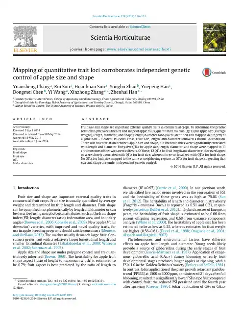
Scientia Horticulturae 174(2014)126–132Contents lists available at ScienceDirectScientiaHorticulturaej o u r n a l h o m e p a g e :w w w.e l s e v i e r.c o m /l o c a t e /s c i h o r tiMapping of quantitative trait loci corroborates independent genetic control of apple size and shapeYuansheng Chang a ,Rui Sun a ,Huanhuan Sun a ,Yongbo Zhao b ,Yuepeng Han c ,Dongmei Chen b ,Yi Wang a ,Xinzhong Zhang a ,∗,Zhenhai Han a ,∗aInstitute for Horticultural Plants,College of Agronomy and Biotechnology,China Agricultural University,Beijing 100193,China bChangli Institute for Pomology,Hebei Academy of Agricultural and Forestry Science,Changli,Heibei 066600,China cWuhan Botanical Garden,The Chinese Academy of Sciences,Wuhan 430074,Chinaa r t i c l ei n f oArticle history:Received 3April 2014Received in revised form 18May 2014Accepted 19May 2014Available online 9June 2014Keywords:Fruit shape Fruit size QTLMalus domesticaa b s t r a c tFruit size and shape are important external quality traits in commercial crops.To determine the genetic relationship between the size and shape of apple fruits,quantitative trait loci (QTLs)for apple size (average weight),length,diameter,and shape (length/diameter ratio)were identified and mapped in progeny of a ‘Jonathan’בGolden Delicious’cross.Fruit size,length,and diameter followed a normal distribution.There was no correlation between apple size and shape,but both variables were significantly correlated with length and diameter.Forty-five QTLs for apple size,length,diameter,and shape were mapped to 13chromosomes of the two parent cultivars.Of these,12QTLs for fruit length and diameter either overlapped or were closely associated with QTLs for fruit size,whereas three co-localized with QTLs for fruit shape.No QTLs for fruit size mapped to the same or neighboring regions as QTLs for fruit shape,suggesting that size and shape are under independent genetic control.©2014Elsevier B.V.All rights reserved.1.IntroductionFruit size and shape are important external quality traits in commercial fruit crops.Fruit size is usually quantified by average weight and determined by fruit length and diameter.Fruit shape can be quantified morphometrically by length and diameter or can be described using morphological attributes,such as the fruit shape index (FSI;length:diameter ratio),indentation area,and boundary angles (Brewer et al.,2006;Gonzalo et al.,2009).New apple (Malus domestica )varieties,with improved and novel quality traits,for use in apple breeding programs should satisfy consumers (Meneses and Orellana,2013).The market usually demands large fruit.Con-sumers prefer fruit with a relatively larger longitudinal length and smaller latitudinal diameter (Tabatabaeefar et al.,2000;Waseem et al.,2002;Sadrnia et al.,2007).Apple size and shape are under polygene control and are quan-titatively inherited (Brown,1960).The heritability for apple fruit shape aspect (ratio of height to maximum width)is estimated to be 0.79;fruit aspect is best predicted by the ratio of length to∗Corresponding authors.Tel.:+861062734391;fax:+861062734391.E-mail addresses:zhangxinzhong999@ (X.Zhang),rschan@ (Z.Han).diameter (R 2=0.97)(Currie et al.,2000).In our previous work,we identified five major genes involved in the segregation of FSI,and the heritability of these genes was as high as 75.0%(Sun et al.,2012).The heritability of length and diameter in strawberry (Fragaria ×ananassa Duch.)is reported as 0.51and 0.21,respec-tively (Lerceteau-Köhler et al.,2012).In hybrid crosses of European pears,the heritability of fruit shape is estimated to be 0.66from parent–offspring regression,and 0.68from variance component analysis (White et al.,2000).The heritability of apple size has been estimated to be as low as 0.33,whereas estimates for fruit weight are higher (0.56–0.61)(Durel et al.,1998;Oraguzie et al.,2001;Alspach and Oraguzie,2002).Phytohormones and environmental factors have different effects on apple fruit length and diameter.Young seeds likely provide a source of gibberellins during the early stages of fruit development (Garcia-Martinez et al.,1987).Application of exoge-nous gibberellic acid (GA 4+7)during blooming or early fruit developmental stages produces longer apples at ripening,with a FSI >1.0in the ‘Golden Delicious’variety (Eccher and Boffelli,1981).In contrast,foliar application of the plant growth retardant paclobu-trazol (PP333)at 1500or 3000ppm,administered 21days after full blooming,resulted in a significantly lower FSI in ripe fruit compared with control fruit;the reduced FSI persisted until the fourth year after spraying (Greene,1986).Foliar application of GA 3or GA 4+7/10.1016/j.scienta.2014.05.0190304-4238/©2014Elsevier B.V.All rights reserved.Y.Chang et al./Scientia Horticulturae174(2014)126–132127counteracted the effect of PP333(Curry and Williams,1983).Con-tinuous fruit growth,from cell division to ripening,is primarily associated with auxin-related cell expansion(Devoghalaere et al., 2012).The harvest weight of apples is closely correlated with seed number(including aborted seeds),and increased fruit weight is attributed to increased cell number rather than cell size(Denne, 1963).Environmental factors can also affect apple fruit shape, specifically temperature and humidity.Shaw(1914)observed that fruit length was longer when temperatures were lower following full bloom.Tromp(1990)reported that the FSI of‘Golden Delicious’was lower in apples grown at a relative humidity between40and 50%than in apples grown at80–90%relative humidity.Developmental rhythms differ for fruit length vs.diameter.The expression of genes important in cell division(e.g.,MdANT1and MdANT2)is high from bloom until15days after full blooming(Dash and Malladi,2012),a period coinciding with active cell division and rapid longitudinal fruit growth(Skene,1966).Quantitative trait loci(QTLs)are important in the investiga-tion of the genetic control of economically valuable traits.Genetic linkage maps enable the identification of chromosome regions con-taining one or more genes associated with QTLs(Meneses and Orellana,2013;Tanksley,1993).Since the generation of thefirst integrated apple linkage map (Rome Beauty×White Angel;Hemmat et al.,1994),several genetic linkage maps have been reported in apple(Conner et al.,1997; Maliepaard et al.,1998;Liebhard et al.,2002,2003;Baldi et al., 2004;Silfverberg-Dilworth et al.,2006;Calenge et al.,2004;Kenis et al.,2008;Zhang et al.,2012).Saturated and high-density genetic linkage maps are useful for genetic research,and many traits have been mapped in apple (Conner et al.,1997;Weeden et al.,1994;Stankiewicz-Kosyl et al., 2005;Fernández-Fernández et al.,2008;Gao et al.,2005).In apple,QTLs for fruit length have been mapped on linkage group(LGs)2,6,15,and17;and QTLs for apple diameter on LGs2, 5,9,10,and17(Kenis et al.,2008).However,mapping results in dif-ferent years(2004and2005)were found to be inconsistent(Kenis et al.,2008).Several QTLs for apple fruit size have been identified in different mapping populations,including‘Fiesta’בDiscovery,’‘Telamon’בBraeburn’,‘Royal Gala’בBraeburn,’and‘Starkrim-son’בGranny Smith’(Liebhard et al.,2003;Kenis et al.,2008; Devoghalaere et al.,2012).We previously mappedfive major gene loci involved in the determination of FSI using bulked segregant analysis in a ‘Jonathan’בGolden Delicious’mapping population;these were located on LGs11,12,and13of the female parent‘Jonathan’,and on LG10of the male parent‘Golden Delicious’(Sun et al.,2012). However,we did not obtain any QTLs without linkage maps at that time.In this study,to clarify the genetic relationships among fruit weight,length,diameter,and FSI,and we analyzed the inheritance of these external quality traits,and identified QTLs associated with them.2.Materials and methods2.1.Plant materialsThe apple cultivars‘Jonathan’(J)and‘Golden Delicious’(G),with ‘Jonathan’as the female parent were crossed in spring2002at the Changli Institute of Pomology(Hebei Province,China)to obtain hybrid progeny.Seedlings were planted in2003at a density of one per0.5m×2m plot,resulting in a J×G F1population of1733 seedlings.After planting,the seedlings were subjected to conven-tionalfield management and pest control procedures(Sun et al., 2012).2.2.PhenotypingApples sufficient for phenotyping were harvested in1162 seedlings in2008.Due to alternate bearing,ripening fruit from971 seedlings were collected in2009.A vernier caliper was used for the measurements of fruit diameter(D)and fruit length(L).The phenotypic value used for further analysis was represented by the average values of at leastfive apples per seedling each year.FSI was calculated using the formula FSI=L/D.Fruit size was recorded as the average fruit weight,and the phenotypic data of fruit size were the average values offive apples,which were determined by weighing the fruit on an analytical balance.2.3.Inheritance analysisTo evaluate the quality of phenotypic data to obtain reliable results of QTL identification,data of fruit length and fruit diame-ter were subjected to analysis of variance(ANOVA,F-test)using Microsoft Excel2003with30randomly selected seedlings,which bear sufficient amounts of fruit(n=10apples per plant)in both 2008and2009.The correlations of fruit length,diameter,shape, and size were analyzed using data collected from983seedlings in 2008and from789seedlings in2009.Inheritance was analyzed using frequency-distribution analysis,Shapiro–Wilk tests(SPSS v.12.0;SPSS Inc.,Chicago,IL,USA),and chi-square tests(Microsoft Excel2003).This protocol has been previously described by Sun et al.(2012).Phenotypic variance(S)was defined as the sum of genotypic variance(Sg)and environmental variance(Se).Heritabil-ity was calculated as(S−Se)/S×100%,and S was calculated using the variance among the30seedlings.Environmental variance was represented by the average variance among the10apples from each seedling(Sun et al.,2012).2.4.QTL analysisQTL analysis was performed using our previously published genetic linkage maps(Zhang et al.,2012),which consisted of 242individuals and251simple sequence repeat(SSR)markers. Phenotypic data on fruit length,diameter,FSI and size for the map-ping population(n=242seedlings)were collected in2008(n=144 seedlings)and2009(n=140seedlings).MapQTL 6.0(Van Ooijen et al.,2009)was used to analyze QTLs.Interval mapping was performed,and the genome-and chromosome-wide threshold for QTL significance of logarithm of odds(LOD)was calculated by performing1000iterations using the MapQTL Permutation Test.The genome-wide threshold was LOD=2.80at the95%confidence interval.3.Results3.1.Phenotype evaluationThere was significant variation in fruit diameter,length,and FSI among the seedlings and between the sampling years,but there were no significant differences among apples from individ-ual seedlings(Table1).Unfortunately,ANOVA could not be used for fruit size because phenotypic data were obtained by averaging the weight of10apples from each seedling.Fruit length and diameter were significantly correlated(r>0.70) in both2008and2009.FSI was positively correlated with fruit length,and negatively correlated with fruit diameter.The abso-lute values of correlation coefficients between FSI and fruit length were larger than those between FSI and fruit diameter,suggesting that length was a more pronounced trait than diameter.Although both length and diameter were positively correlated with fruit size, the correlation was stronger for diameter,indicating that fruit size128Y.Chang et al./Scientia Horticulturae 174(2014)126–132Fig.1.Frequency distributions of fruit length,diameter,and size (weight)in progenies from the ‘Jonathan’בGolden Delicious’hybrid cross.Phenotypic data were collected in 2008and 2009.The parental values are indicated on the figures with vertical dash lines.(weight)was more a function of diameter than of length.No signif-icant correlation was detected between FSI and fruit size (Table 2).Fruit size,length,and diameter followed normal distribution patterns in both sampling years,and they showed features typical of quantitative traits controlled by polygenes without major gene segregation (Fig.1).The broad-sense heritability of fruit length and diameter were estimated as 91%and 93%,respectively in 2008;and as 82%and 85%in 2009.These values indicated that environmental effects had a greater effect on fruit quality in 2009(Table 3).3.2.QTL analysisNineteen QTLs for fruit size,shape,length,and diameter were identified at the whole-genome level based on a LOD thresh-old ≥2.80in both sampling years (Table 4).Twenty-six additionalTable 1F -tests of phenotypic traits in apple fruit.VariationTraitYearFF 0.01Seedlings Length 2008106.62* 1.78200947.57* 1.78Diameter2008142.01* 1.78200960.69*1.78ReplicatesLength20080.22 2.4720090.70 2.47Diameter20080.147 2.4720090.542.47YearsLength 56.53* 6.68Diameter23.05*6.68*Significant difference at P ≤0.01as determined using Duncan’s test.QTLs were identified,based on a permutation test at P =0.05,at the single-chromosome-based LOD threshold (Table 4,Fig.2).Of these,eight QTLs related to fruit length were detected in 2008;no QTLs for fruit length were detected in 2009.Eleven and two QTLs for fruit size were identified in 2008and 2009,respec-tively.Nine QTLs in 2008and two QTLs in 2009for fruit diameter mapped onto the two parental linkage groups.In addition,we also detected seven and six QTLs associated with FSI in 2008and 2009,respectively.For FSI,one QTL,fsij08.11.2/fsij09.11on LG11of the female parent ‘Jonathan,’and one QTL fsig08.15/fsig09.15.1in the male parent ‘Golden Delicious’were observed in both years (Fig.2).Four QTLs for fruit size,four for diameter,and three for length co-localized and clustered on chromosome 8of ‘Golden Delicious.’The fszg08.11.1QTL for fruit size was tightly linked to flg08.11forTable 2Correlations between apple length,diameter,shape index,and size in a ‘Jonathan’בGolden Delicious’hybrid population.Fruit traitFruit lengthFruit diameterFruit shape2008Fruit diameter 0.77*Fruit shape 0.48*−0.19*Fruit size0.76*0.87*−0.0332009Fruit diameter 0.76*Fruit shape 0.42*−0.27*Fruit size0.78*0.89*−0.084983seedlings in 2008and 789in 2009were used to analyze the correlations of fruit length,diameter,shape and size (r 0.05=0.0625and r 0.01=0.082in 2008;r 0.05=0.07and r 0.01=0.09in 2009).*Significance at P =0.05.Y.Chang et al./Scientia Horticulturae174(2014)126–132129 Table3Estimated heredity parameters for apple length and diameter in a‘Jonathan’בGolden Delicious’hybrid population.Trait Year Average±SD(mm)Population variance(S)Genetic variance(Sg)Environmental variance(Se)Heritability(%) Fruit length200858.66±5.48123.41112.4310.9891.10 200952.88±4.5828.3823.24 5.1481.89Fruit diameter200868.70±5.69156.63145.9610.6793.20 200963.27±5.1540.3334.39 5.9485.30length and to fdg08.11for diameter on LG11of‘Golden Delicious’(Table4,Fig.2).The QTL fszj08.15(fruit size)overlappedflj08.15 (fruit length)exactly on chromosome15of‘Jonathan’.The fszg08.3 QTL for fruit-size coincided with fdg08.11.3(fruit diameter)and QTL fszj08.5(fruit size),and partially overlapped fdj08.5(fruit diame-ter)on LG5of‘Jonathan’(Table4,Fig.2).For FSI,fsij08.4partially overlappedflj08.4(fruit length)on LG4of Jonathan;fsij09.9was co-localized with fdj09.9on LG9;and fsij08.17was closely linked to flj08.17on LG17of‘Jonathan’(Table4,Fig.2).4.DiscussionFruit size and shape indices were closely associated with length and diameter,whereas the inheritance of fruit size,shape,length, and diameter differed.The normal distribution of phenotypic traits suggests that apple length,diameter,and size are under polygenetic control.However,variation in FSI is associated with segregation in both major genes and polygenes,and the heritability of major genes was found to be as high as75%(Sun et al.,2012).Table4Quantitative trait loci(QTLs)and mapping information for apple size,shape,length,and diameter in segregated progeny of‘Jonathan’בGolden Delicious’.Trait Year QTL LG Location Nearest marker LOD Contribution to totalvariance(%)Fruit length2008flj08.15J150.000WBGCAS50 3.5010.10flj08.17J17-20.000NZmsEB137525 2.337.60flj08.4J40.000Hi23g08 2.01 6.20flj08.8J871.700Hi23g12 1.797.30flg08.8.1G869.141H20b03 3.9812.10flg08.8.2G837.552BACSSR46 3.0411.80flg08.8.3G830.644CTG1069672 3.3013.00flg08.11G1116.788CH05c02 2.347.70Fruit diameter2008fdj08.5J591.033NZmsCN898349 2.809.20fdj08.13J1321.582CTG1075622 2.087.20fdg08.2G258.212CH03d10 2.387.30fdg08.3G382.408WBGCAS27 2.258.10fdg08.8.1G868.660Hi20b03 3.1710.1fdg08.8.2G853.250CH05a02 3.0212.5fdg08.8.3G837.552BACSSR46 2.8510.90fdg08.8.4G830.644CTG1069672 3.0311.30fdg08.11G1120.788BACSSR10 2.539.202009fdj09.9J927.391CTG1067792 2.739.10fdg09.4G4 5.000CH01b01b 1.80 6.30Fruit shape index2008fsij08.4J40.000Hi23g08 2.878.40fsij08.17J17-2 5.000CN938125 1.91 6.20fsig08.15G15-1 1.000CH02c09 2.598.00fsij08.11.1J1114.813Hi23d02 4.0012.80fsij08.11.2J117.371CH02d12 3.4210.30fsij08.11.3J11 3.000CH02d08 3.7613.70fsij08.5J57.000CN881672 1.817.702009fsij09.9J924.391CTG1067792 2.659.20fsij09.13J1332.087CTG1075622 2.2110.00fsij09.7J715.069CTG1060504 1.817.20fsig09.15.1G15-1 3.000CH02c09 1.95 6.70fsig09.15.2G15-151.249NZmsEB117266 1.85 5.50fsij09.11J117.371CH02d12 4.0210.20Fruit size2008fszg08.8.1G869.141Hi20b03 4.2912.80fszg08.8.2G851.250CH04g12 3.0712.60fszg08.8.3G837.552BACSSR46 3.1311.50fszg08.8.4G828.644CTG1069672 3.3112.60fszg08.11.1G1124.788BACSSR10 2.979.70fszg08.11.2G119.930CH04a12 2.447.30fszg08.11.3G110.000CH02d08 2.147.10fszj08.5J595.033Hi02a03 2.517.7fszj08.15J150WBGCAS50 2.227.2fszj08.12J1257.944CH03c02 2.019.6fszg08.3G384.408WBGCAS27 1.72 6.42009fszg09.12G1245.311WBGCAS37 2.02 6.7fszg09.14G1494.33NZmsEB146613 1.858.9LG:linkage group;LOD:logarithm of odds.QTLs detected at whole-genome LOD threshold≥2.8are indicated in bold fonts.130Y.Chang et al./Scientia Horticulturae 174(2014)126–132Fig.2.Internal mapping of quantitative trait loci (QTLs)for fruit length,diameter,shape index (FSI),and size using the ‘Jonathan’בGolden Delicious’hybrid population.The letters J and G on the top of the linkage maps represent the maternal parent ‘Jonathan’and pollen parent ‘Golden Delicious’,respectively.The number following J and G indicates the number of linkage groups.Homologs between parents on corresponding linkage groups (LGs)are joined to each other with solid black lines.The solid color bars indicate the QTLs identified on the most likely position of the linkage groups,while the thin lines represent the confidence interval at the 95%level.QTLs for fruit length,diameter,size,and FSI are marked by the black,blue,red,and yellow color bars,respectively.F11-1and F11-2,on LG11of ‘Jonathan’,represent the two major gene loci for FSI detected by Sun et al.(2012).(For interpretation of the references to color in this legend,the reader is referred to the web version of the article.)Our findings contrasted with previous reports that apple fruit size is a quantitative trait with relatively low heritability (0.33–0.61)(Durel et al.,1997;Oraguzie et al.,2001;Alspach and Oraguzie,2002).The heritability of fruit length and diameter was relatively high (82–93%)during the two years of evaluation.Both FSI and fruit size correlated with fruit length and diameter.QTLs for closely correlated traits should map to the same or simi-lar positions (Paterson et al.,1991;Kenis et al.,2008).Thus,QTLs associated with FSI or fruit size,at least in part,should overlap or be linked to those for fruit length and diameter.Indeed,the three QTLs for fruit size (fszg08.8.1,fszg08.8.3,and fszg08.8.4)completely overlapped QTLs for fruit length (flg08.8.1,flg08.8.3,and flg08.8.4),and those for fruit diameter (fdg08.8.1,fdg08.8.3,and fdg08.8.4).In ‘Telamon’and ‘Braeburn’progeny,QTLs for apple weight,height,and diameter on LG17partially overlapped with QTLs for fruit height and diameter on LG2.Furthermore,year-stable QTLs for fruit weight and diameter overlapped on LG10of the two par-ents (Kenis et al.,2008).Similarly,the QTL for FSI (fsij08.4)precisely overlapped the one for fruit length (flj08.4),whereas fsij09.9and fsij08.17for FSI were closely linked to fdj09.9and flj08.17,respec-tively.These co-localizations confirmed the correlation analysis that indicated that fruit length strongly affects FSI.In our hybrid population,QTLs for fruit length (on LGs 15and 17)and diameter(on LGs 2,5,and 9)were located on the same LGs as QTLs in the ‘Telamon’בBraeburn’cross (Kenis et al.,2008).Using two map-ping populations,Devoghalaere et al.(2012)identified six QTLs for fruit size,on LGs 5,8,11,15,16,and 17;of these,QTLs on LGs 8and 15were conserved across both populations.In hybrid populations derived from European and Chinese pears,QTLs for FSI,weight,and length co-localized on LG8;interestingly,some QTLs clustered on LG7of the female parent (Zhang et al.,2013).However,we did not detect significant correlations between FSI and fruit size.Thus,the QTLs for these traits did not map close to each other on the same chromosomes.Rather,QTLs for FSI over-lapped with or were linked to QTLs for fruit length and diameter on chromosomes that were not linked to fruit size,thus demonstrat-ing that FSI and fruit size are controlled by different genes.Such independent genetic control differs fundamentally from other fruit species,such as pear (Zhang et al.,2013).In muskmelon (Cucumis melo L.),the major QTL for fruit shape (fs2.2)is co-localized with a major gene (andromonoecious );this effect is detectable in com-parisons of ovary and fruit length,but not ovary and fruit width (Périn et al.,2002).Another major QTL for fruit shape,fs12.1,co-segregates with another major gene,pentamerous ,and this effect is detectable in comparisons of ovary and fruit width,but not ovary and fruit length (Périn et al.,2002).Y.Chang et al./Scientia Horticulturae174(2014)126–132131We observed a significant correlation between fruit length and diameter,and a close relationship between fruit diameter and size. Four QTLs for fruit diameter,compared with only one QTL for fruit length,co-segregated with or closely linked to QTLs for fruit size. Four QTLs also contributed simultaneously to fruit size,length, and diameter.Instability of QTLs between different years of detec-tion has been reported for many species(Liebhard et al.,2003; Zhang et al.,2013).However,only two QTLs,fsij08.11.2/fsij09.11 and fsig08.15/fsig09.15.1,were stable across the two-year study.The variation in fruit length and diameter between the sampling years indicates that environmental effects or genotype–environment interactions affect the robustness of QTLs between years.Kenis et al.(2008)also observed that QTLs for fruit weight,diameter,and height differed among years.QTL-mapping software provides a powerful tool for detecting major genes for qualitative and quantitative traits(Jones et al., 1997).Our previous study used the same data sets to identifyfive major gene loci involved in apple FSI(Sun et al.,2012).Of thesefive loci,F11-1(Fig.2),flanked by CH02d08and CH04a12,mapped to the same region as the year-stable QTL fsij08.11.2/fsij09.11at7.371 cM on chromosome11of the female parent‘Jonathan’,closest to CH02d12.The major gene locus F13was located in the same region as the QTL fsij09.13(Sun et al.,2012).In the apple genome,more than10genes related to fruit growth and development,including genes involved in cell division and auxin signaling,are scattered in the region of CH02d12,at7.371 cM on LG11.An auxin response factor gene,ARF106,which modu-lates cell division and expansion,is co-localized with a stable QTL for fruit weight in duplicated regions on LGs8and15of the apple genome(Devoghalaere et al.,2012).In conclusion,45QTLs for apple fruit size,shape,length,and diameter were identified from a‘Jonathan’×’Golden Delicious’population.Of the19QTLs for fruit length and diameter,12over-lapped with or tightly linked to QTLs for fruit size,and another three co-localized with QTLs for fruit shape.None of the QTLs for fruit size mapped to the same region as QTLs for fruit shape,indicating that fruit size and shape are under independent genetic control.AcknowledgmentsThis work was supported by the Hi-Tech Research and Devel-opment(863)Program of China(2011AA001204);National Special Funds for Scientific Research on Public Causes(Agriculture)Project 200903044;Modern Agricultural Industry Technology System (Apple)(CARS-28);and Key Laboratory of Biology and Genetic Improvement of Horticultural Crops(Nutrition and Physiology), Ministry of Agriculture,P.R.China.Appendix A.Supplementary dataSupplementary data associated with this article can be found,in the online version,at /10.1016/j.scienta. 2014.05.019.ReferencesAlspach,P.A.,Oraguzie,N.C.,2002.Estimation of genetic parameters of apple(Malus domestica)fruit quality from open-pollinated families.New Zeal.J.Crop Hortic.Sci.30,219–228.Baldi,P.,Patocchi,A.,Zini,E.,Toller,C.,Velasco,R.,Komjanc,M.,2004.Cloning and linkage mapping of resistance gene homologues in apple.Theor.Appl.Genet.109,231–239.Brewer,M.T.,Lang,L.,Fujimura,K.,Dujmovic,N.,Gray,S.,Van der Knaap,E.,2006.Development of a controlled vocabulary and software application to analyze fruit shape variation in tomato and other plant species.Plant Physiol.141,15–25. Brown,A.G.,1960.The inheritance of shape,size and season of ripening in progenies of the cultivated apple.Euphytica9,327–337.Calenge,F.,Faure,A.,Goerre,M.,Gebhardt,C.,Van de Weg,W.E.,Parisi,L.,Durel,C.E.,2004.Quantitative trait loci(QTL)analysis reveals both broad-spectrumand isolate-specific QTL for scab resistance in an apple progeny challenged with eight isolates of Venturia inaequalis.Phytopathology94,370–379.Conner,P.J.,Brown,S.K.,Weeden,N.F.,1997.Randomly amplified polymorphic DNA-based genetic linkage maps of three apple cultivars.J.Am.Soc.Hortic.Sci.122, 350–359.Curry,E.A.,Williams,M.W.,1983.Promalin or GA increase pedicel and fruit length and leaf size of‘Delicious’apples treated with paclobutrazol.Hortscience18, 214–215.Currie,A.J.,Ganeshanandam,S.,Noiton,D.A.,Garrick,D.,Shelbourne,C.J.A.,Oraguzie, N.,2000.Quantitative evaluation of apple(Malus×domestica Borkh.)fruit shape by principal component analysis of Fourier descriptors.Euphytica111,221–227. Dash,M.,Malladi,A.,2012.The AINTEGUMENTA genes,MdANT1and MdANT2,are associated with the regulation of cell production during fruit growth in apple (Malus×domestica Borkh.).BMC Plant Biol.12,98.Denne,M.P.,1963.Fruit development and some tree factors affecting it.New Zeal.J.Bot.1,265–294.Devoghalaere,F.,Doucen,T.,Guitton,B.,Keeling,J.,Payne,W.,Ling,T.J.,Ross,J.J., Hallett,I.C.,Gunaseelan,K.,Dayatilake,G.A.,Diak,R.,Breen,K.C.,Tustin,D.S., Costes,E.,Chagne,D.,Schaffer,R.J.,David,K.M.,2012.A genomics approach to understanding the role of auxin in apple(Malus×domestica)fruit size control.BMC Plant Biol.12,7.Durel,C.E.,Laurens,F.,Fouillet,A.,Lespinasse,Y.,1998.Utilization of pedigree infor-mation to estimate genetic parameters from large unbalanced data sets in apple.Theor.Appl.Genet.96,1077–1085.Eccher,T.,Boffelli,G.,1981.Effect of dose and time of application of GA on russeting fruit set and shape of Golden Delicious apple.Sci.Hortic.14, 307–314.Fernández-Fernández,F.,Evans,K.M.,Clarke,J.B.,Govan,C.L.,James,C.M.,Mariˇc,S., Tobutt,K.R.,2008.Development of an STS map of an interspecific progeny of Malus.Tree Genet.Genomics4,469–479.Gao,Z.S.,Van de Weg,W.E.,Schaart,J.G.,Van der Meer,I.M.,Kodde,L.,Laimer,M., Breiteneder,H.,Hoffmann-Sommergruber,K.,Gilissen,L.J.W.J.,2005.Linkage map positions and allelic diversity of two Mal d3(non-specific lipid transfer protein)genes in the cultivated apple(Malus domestica).Theor.Appl.Genet.110,479–491.Garcia-Martinez,J.L.,Sponsel,V.M.,Gaskin,P.,1987.Gibberellins in developing fruits of Pisum sativum cv.Alaska:studies on their role in pod growth and seed devel-opment.Planta170,130–137.Greene,D.W.,1986.Effect of paclobutrazol and analogs on growth yield,fruit quality, and storage of‘Delicious’apples.J.Am.Soc.Hortic.Sci.111,328–332. Gonzalo,M.J.,Brewer,M.T.,Anderson,C.,Sullivan,D.,Gray,S.,Van der Knaap,E.,2009.Tomato fruit shape analysis using morphometric and morphologyattributes implemented in tomato analyzer software program.J.Am.Soc.Hortic.Sci.134,77–87.Hemmat,M.,Weeden,N.F.,Manganaris,A.G.,Lawson,D.M.,1994.Molecular marker linkage map for apple.J.Hered.85,4–11.Jones,N.,Ougham,H.,Thomas,H.,1997.Markers and mapping:we are all geneticists now.New Phytol.137,165–177.Kenis,K.,Keulemans,J.,Davey,M.W.,2008.Identification and stability of QTLs for fruit quality traits in apple.Tree Genet.Genomes4,647–661.Lerceteau-Köhler,E.,Moing,A.,Guérin,G.,Renaud,C.,Petit,A.,Rothan,C.,Denoyes,B.,2012.Genetic dissection of fruit quality traits in the octoploid cultivatedstrawberry highlights the role of homoeo-QTL in their control.Theor.Appl.Genet.124,1059–1077.Liebhard,R.,Gianfranceschi,L.,Koller,B.,Ryder,C.D.,Tarchini,R.,Van De Weg,E., Gessler,C.,2002.Development and characterisation of140new microsatellites in apple(Malus×domestica Borkh.).Mol.Breeding10,217–241.Liebhard,R.,Kellerhals,M.,Pfammatter,W.,Jertmini,M.,Gessler,C.,2003.Mapping quantitative physiological traits in apple(Malus×domestica Borkh.).Plant Mol.Biol.52,511–526.Maliepaard,C.,Alston,F.H.,Van Arkel,G.,Brown,L.M.,Chevreau,E.,Dunemann,F., Evans,K.M.,Gardiner,S.,Guilford,P.,Van Heusden,A.W.,Janse,J.,Laurens,F., Lynn,J.R.,Manganaris,A.G.,Den Nijs,A.P.M.,Periam,N.,Rikkerink,E.,Roche, P.,Ryder,C.,Sansavini,S.,Schmidt,H.,Tartarini,S.,Verhaegh,J.J.,Vrielink-van Ginkel,M.,King,G.J.,1998.Aligning male and female linkage maps of apple (Malus pumila Mill.)using multi-allelic markers.Theor.Appl.Genet.97,60–73. Meneses,C.,Orellana,A.,ing genomics to improve fruit quality.Biol.Res.46,347–352.Oraguzie,N.C.,Hofstee,M.E.,Brewer,L.R.,Howard,C.,2001.Estimation of genetic parameters in a recurrent selection program in apple.Euphytica118,29–37. Paterson,A.H.,Damon,S.,Hewitt,J.D.,Zamir,D.,Rabinowitch,H.D.,Lincoln,S.E., Lander,E.S.,Tanksley,S.D.,1991.Mendelian factors underlying quantitative traits in tomato:comparison across species,generations,and environments.Genetics127,181–197.Périn,C.,Hagen,L.S.,Giovinazzo,N.,Besombes,D.,Dogimont,C.,Pitrat,M.,2002.Genetic control of fruit shape acts prior to anthesis in melon(Cucumis melo L.).Mol.Genet.Genomics266,933–941.Sadrnia,H.,Rajabipour,A.,Jafary,A.,Javadi,A.,Mostofi,A.,2007.Classification and analysis of fruit shapes in long type watermelon using image processing.Int.J.Agric.Biol.9,68–70.Shaw,J.K.,1914.A study in variation in apples.Mass.Agric.Exp.Stn.Bull.149,21–36. Silfverberg-Dilworth,E.,Matasci,C.L.,Van de Weg,W.E.,Van Kaauwen,M.P.W., Walser,M.,Kodde,L.P.,Soglio,V.,Gianfranceschi,L.,Durel, C.E.,Costa, F., Yamamoto,T.,Koller,B.,Gessler,C.,Patocchi,A.,2006.Microsatellite markers spanning the apple(Malus×domestica Borkh.)genome.Tree Genet.Genomes2, 202–224.。

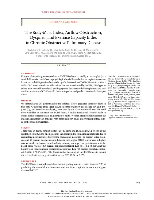
n engl j med 350;10march 4, 2004 The new england journal of medicine1005The Body-Mass Index, Airflow Obstruction, Dyspnea, and Exercise Capacity Index in Chronic Obstructive Pulmonary DiseaseBartolome R. Celli, M.D., Claudia G. Cote, M.D., Jose M. Marin, M.D., Ciro Casanova, M.D., Maria Montes de Oca, M.D., Reina A. Mendez, M.D.,Victor Pinto Plata, M.D., and Howard J. Cabral, Ph.D.From the COPD Center at St. Elizabeth’s Medical Center, Tufts University School of Medicine, Boston (B.R.C., V .P.P.); Bay Pines Veterans Affairs Medical Center, Bay Pines,Fla. (C.G.C.); Hospital Miguel Servet, Zara-goza, Spain (J.M.M.); H ospital Nuestra Senora de La Candelaria, Tenerife, Spain (C.C.); Hospital Universitario de Caracas and Hospital Jose I. Baldo, Caracas, Vene-zuela (M.M.O., R.A.M.); and Boston Uni-versity School of Public H ealth, Boston (H.J.C.). Address reprint requests to Dr.Celli at Pulmonary and Critical Care Medi-cine, St. Elizabeth’s Medical Center, 736Cambridge St., Boston, MA 02135, or at bcelli@.N Engl J Med 2004;350:1005-12.Copyright © 2004 Massachusetts Medical Society.backgroundChronic obstructive pulmonary disease (COPD) is characterized by an incompletely re-versible limitation in airflow. A physiological variable — the forced expiratory volume in one second (FEV 1 ) — is often used to grade the severity of COPD. However, patients with COPD have systemic manifestations that are not reflected by the FEV 1 . We hypoth-esized that a multidimensional grading system that assessed the respiratory and sys-temic expressions of COPD would better categorize and predict outcome in these pa-tients.methodsWe first evaluated 207 patients and found that four factors predicted the risk of death in this cohort: the body-mass index (B), the degree of airflow obstruction (O) and dys-pnea (D), and exercise capacity (E), measured by the six-minute–walk test. We used these variables to construct the BODE index, a multidimensional 10-point scale in which higher scores indicate a higher risk of death. We then prospectively validated the index in a cohort of 625 patients, with death from any cause and from respiratory caus-es as the outcome variables.resultsThere were 25 deaths among the first 207 patients and 162 deaths (26 percent) in the validation cohort. Sixty-one percent of the deaths in the validation cohort were due to respiratory insufficiency, 14 percent to myocardial infarction, 12 percent to lung can-cer, and 13 percent to other causes. Patients with higher BODE scores were at higher risk for death; the hazard ratio for death from any cause per one-point increase in the BODE score was 1.34 (95 percent confidence interval, 1.26 to 1.42; P<0.001), and the hazard ratio for death from respiratory causes was 1.62 (95 percent confidence inter-val, 1.48 to 1.77; P<0.001). The C statistic for the ability of the BODE index to predict the risk of death was larger than that for the FEV 1 (0.74 vs. 0.65).conclusionsThe BODE index, a simple multidimensional grading system, is better than the FEV 1at predicting the risk of death from any cause and from respiratory causes among pa-tients with COPD.The new england journal of medicine1006hronic obstructiv e pulmonarydisease (COPD), a common disease char-acterized by a poorly reversible limitationin airflow,1 is predicted to be the third most fre-quent cause of death in the world by 2020.2 Therisk of death in patients with COPD is often gradedwith the use of a single physiological variable, theforced expiratory volume in one second (FEV1).1,3,4However, other risk factors, such as the presenceof hypoxemia or hypercapnia,5,6 a short distancewalked in a fixed time,7 a high degree of functionalbreathlessness,8 and a low body-mass index (theweight in kilograms divided by the square of theheight in meters),9,10 are also associated with anincreased risk of death. We hypothesized that a mul-tidimensional grading system that assessed the res-piratory, perceptive, and systemic aspects of COPDwould better categorize the illness and predict theoutcome than does the FEV1 alone. We used datafrom an initial cohort of 207 patients to identifyfour factors that predicted the risk of death: thebody-mass index (B), the degree of airflow ob-struction (O) and functional dyspnea (D), and exer-cise capacity (E) as assessed by the six-minute–walk test. We then integrated these variables into amultidimensional index — the BODE index — andvalidated the index in a second cohort of 625 pa-tients, with death from any cause and death from859 outpatients with a wide range in the severityof COPD were recruited from clinics in the UnitedStates, Spain, and Venezuela. The study was ap-proved by the human-research review board at eachsite, and all patients provided written informed con-sent. COPD was defined by a history of smokingthat exceeded 20 pack-years and a ratio of FEV1 toforced vital capacity (FVC) of less than 0.7 measured20 minutes after the administration of albuterol.1All patients were in clinically stable condition andreceiving appropriate therapy. Patients who werereceiving inhaled oxygen had to have been takinga stable dose for at least six months before studyentry. The exclusion criteria were an illness otherthan COPD that was likely to result in death withinthree years; asthma, defined as an increase in theFEV1 of more than 15 percent above the base-linevalue or of 200 ml after the administration of a bron-chodilator; an inability to take the lung-functionand six-minute–walk tests; a myocardial infarctionwithin the preceding four months; unstable angi-na; or congestive heart failure (New York Heart As-sociation class III or IV).variables selected for the bode indexWe determined the following variables in the first207 patients who were recruited between 1995 and1997: age; sex; pack-years of smoking; FVC; FEV1,measured in liters and as a percentage of the pre-dicted value according to the guidelines of theAmerican Thoracic Society11; the best of two six-minute–walk tests performed at least 30 minutesapart12; the degree of dyspnea, measured with theuse of the modified Medical Research Council(MMRC) dyspnea scale13; the body-mass index9,10;the functional residual capacity and inspiratorycapacity11; the hematocrit; and the albumin level.The validated Charlson index was used to deter-mine the degree of comorbidity. This index hasbeen shown to predict mortality.14 The differenc-es in these values between survivors and nonsur-vivors are shown in Table 1.Each of these possible explanatory variableswas independently evaluated to determine its as-sociation with one-year mortality in a stepwise for-ward logistic-regression analysis. A subgroup offour variables had the strongest association — thebody-mass index, FEV1 as a percentage of the pre-dicted value, score on the MMRC dyspnea scale,and the distance walked in six minutes (general-ized r2=0.21, P<0.001) — and these were includ-ed in the BODE index (Table 2). All these variablespredict important outcomes, are easily measured,and may change over time. We chose the post-bron-chodilator FEV1 as a percent of the predicted value,classified according to the three stages identifiedby the American Thoracic Society, because it can beused to predict health status,15 the rate of exacer-bation of COPD,16 the pharmacoeconomic costs ofthe disease,17 and the risk of death.18,19 We chosethe MMRC dyspnea scale because it predicts thelikelihood of survival among patients with COPD8and correlates well with other scales and health-status scores.20,21 We chose the six-minute–walktest because it predicts the risk of death in patientswith COPD,7 patients who have undergone lung-reduction surgery,22 patients with cardiomyopa-thy,23 and those with pulmonary hypertension.24In addition, the test has been standardized,12 theclinically significant thresholds have been deter-mined,25 and it can be used to predict resource uti-cn engl j med 350; march 4, 2004n engl j med 350;10march 4, 2004 a multidimensional grading system in chronic obstructive pulmonary disease1007lization. 26 Finally, there is an inverse relation be-tween body-mass index and survival 9,10 that is not linear but that has an inflection point, which was 21 in our cohort and in another study. 10validation of the bode indexThe BODE index was validated prospectively in two ways in a different cohort of 625 patients who were recruited between January 1997 and January 2003. First, we used the empirical model: for each threshold value of FEV 1 , distance walked in six min-utes, and score on the MMRC dyspnea scale shown in Table 2, the patients received points ranging from 0 (lowest value) to 3 (maximal value). For body-mass index the values were 0 or 1, because of the unique relation between body-mass index and survival described above. The points for each varia-ble were added, so that the BODE index ranged from 0 to 10 points, with higher scores indicating a greater risk of death. In an exploratory analysis, the various components of the BODE index were as-signed different weights, with no corresponding increase in predictive value.study protocolIn the cohort, patients were evaluated with the use of the BODE index within six weeks after enroll-ment and were seen every three to six months for at least two years or until death. The patient and family were contacted if the patient failed to return for appointments. Death from any cause and from specific respiratory causes was recorded. The cause of death was determined by the investigators at each site after reviewing the medical record and death certificate.statistical analysisData for continuous variables are presented as means ± SD. Comparison among the three coun-tries was completed with the use of one-way analy-sis of variance. The differences between survivors and nonsurvivors in pulmonary-function variables and other pertinent characteristics were established with the use of t-tests for independent samples.To evaluate the capacity of the BODE index to pre-dict the risk of death, we performed Cox propor-tional-hazards regression analyses. 27 We estimat-ed the hazard ratio, 95 percent confidence interval,and P value for the BODE score, before and after adjustment for coexisting conditions as measured by the Charlson index. We repeated these analyses using the BODE index as the predictor of interest in*FVC denotes forced vital capacity, FEV 1 forced expiratory volume in one sec-ond, and FRC functional residual capacity.†Scores on the modified Medical Research Council (MMRC) dyspnea scale can range from 0 to 4, with a score of 4 indicating that the patient is too breathless to leave the house or becomes breathless when dressing or undressing.‡The body-mass index is the weight in kilograms divided by the square of the height in meters.§Scores on the Charlson index can range from 0 to 33, with higher scores indi- cating more coexisting conditions.*The cutoff values for the assignment of points are shown for each variable. The total possible values range from 0 to 10. FEV 1 denotes forced expiratory volume in one second.†The FEV 1 categories are based on stages identified by the American Thoracic Society.‡Scores on the modified Medical Research Council (MMRC) dyspnea scale can range from 0 to 4, with a score of 4 indicating that the patient is too breathless to leave the house or becomes breathless when dressing or undressing.§The values for body-mass index were 0 or 1 because of the inflection point in the inverse relation between survival and body-mass index at a value of 21.The new england journal of medicine1008dummy-variable form, using the first quartile as thereference group. These analyses yielded estimatesof risk similar to those obtained from analyses us-ing the BODE score as a continuous variable. Thus,we focus our presentation on the predictive charac-teristics of the BODE index and present only bivari-ate results for survival according to quartiles of theBODE index in a Kaplan–Meier analysis. The statis-tical significance was evaluated with the use of thelog-rank test. We also performed bivariate analysison the stage of COPD according to the validatedstaging system of the American Thoracic Society.3In the Cox regression analysis, we assessed thereliability of the model with the body-mass index,degree of airflow obstruction and dyspnea, and ex-ercise capacity score as the predictor of the time todeath by computing bootstrap estimates using thefull sample for the hazard ratio and its 95 percentconfidence interval (according to the percentilemethod). This approach has the advantage of notrequiring that the data be split into subgroups andis more precise than alternative methods, such ascross-validation.28Finally, in order to determine how much moreprecise the BODE index is than the FEV1 alone, wecomputed the C statistics29 for a model containingFEV1 or the BODE score as the sole independentvariable. We compared the survival times and esti-mated the probabilities of death up to 52 months.In these analyses, the C statistic is a mathematicalfunction of the sensitivity and specificity of theBODE index in classifying patients by means of theCox model as either dying or surviving. The nullvalue for the C statistic is 0.5, with a maximum of29patients (Tables 3 and 4) with all degrees of severityof COPD. The FEV1 was slightly lower among pa-tients in the United States than among those in Ven-ezuela or Spain. The U.S. patients also had morefunctional impairment, more severe dyspnea, andmore coexisting conditions. The 27 patients (4 per-cent) lost to follow-up were evenly distributed ac-cording to the severity of COPD and did not differsignificantly from the rest of the cohort with respectto any measured characteristic. There were 162deaths (26 percent) over a median follow-up of 28months (range, 4 to 68). The majority of patients(61 percent) died of respiratory insufficiency, 14percent died of myocardial infarction, 12 percentof lung cancer, and the rest of miscellaneouscauses. The BODE score was lower among survi-vors than among those who died from any cause(3.7±2.2 vs. 5.9±2.6, P<0.005). The score was alsolower among survivors than among those whodied of respiratory causes, and the difference be-tween the scores was larger (3.6±2.2 vs. 6.7±2.3,P<0.001).Table 5 shows the BODE index as a predictor ofdeath from any cause after correction for coexistingconditions. There were significantly more deathsin the United States (32 percent) than in Spain (15percent) or Venezuela (13 percent) (P<0.001). How-ever, when the analysis was done separately foreach country, the predictive power of the BODE in-dex was similar; therefore, the data are presentedtogether. Table 5 shows that the BODE index wasalso a predictor of death from respiratory causesafter correction for coexisting conditions (hazardratio, 1.63; 95 percent confidence interval, 1.48 to1.80; P<0.001). The Kaplan–Meier analysis of sur-*Because of rounding, percentages do not total 100. Thethree stages of chronic obstructive pulmonary disease(COPD) were defined by the American Thoracic Society.FEV1 denotes forced expiratory volume in one second.†Higher scores on the body-mass index, degree of airflowobstruction and dyspnea, and exercise capacity (BODE)index indicate a greater risk of death. Quartile 1 was de-fined by a score of 0 to 2, quartile 2 by a score of 3 to 4,quartile 3 by a score of 5 to 6, and quartile 4 by a scoreof 7 to 10.n engl j med 350; march 4, 2004n engl j med 350;10march 4, 2004 a multidimensional grading system in chronic obstructive pulmonary disease1009vival (Fig. 1A) shows that each quartile increase in the BODE score was associated with increased mor-tality (P<0.001). Thus, the highest quartile (a BODE score of 7 to 10) was associated with a mortality rate of 80 percent at 52 months. These same data are shown in Figure 1B in relation to the severity of COPD according to the staging system of the Amer-ican Thoracic Society. The C statistic for the ability of the BODE index to predict the risk of death was 0.74, as compared with a value of 0.65 with the use of FEV 1 alone (expressed as a percentage of the pre-dicted value). The computation of 2000 bootstrap samples for these data and estimation of the haz-ard ratios for death indicated that for each one-point increment in the BODE score the hazard ratio for death from any cause was 1.34 (95 percent confi-dence interval, 1.26 to 1.42) and the hazard ratio for death from a respiratory cause was 1.62 (95 per-the BODE index — and validated its use by show-ing that it is a better predictor of the risk of death from any cause and from respiratory causes than is the FEV 1 alone. We believe that the BODE index is useful because it includes one domain that quan-tifies the degree of pulmonary impairment (FEV 1 ),one that captures the patient’s perception of symp-toms (the MMRC dyspnea scale), and two indepen-dent domains (the distance walked in six minutes and the body-mass index) that express the systemic consequences of COPD. The FEV 1 is essential for the diagnosis and quantification of the respirato-ry impairment resulting from COPD. 1,3,4 In addi-tion, the rate of decline in FEV 1 is a good marker of disease progression and mortality. 18,19 Howev-er, the FEV 1 does not adequately reflect all the sys-temic manifestations of the disease. For example,the FEV 1 correlates weakly with the degree of dys-pnea, 20 and the change in FEV 1 does not reflect the rate of decline in patients’ health. 30 More impor-tant, prospective observational studies of patients with COPD have found that the degree of dyspnea 8 and health-status scores 31 are more accurate pre-dictors of the risk of death than is the FEV 1 . Thus,although the FEV 1 is important to obtain and essen-tial in the staging of disease in any patient with COPD, other variables provide useful information that can improve the comprehensibility of the eval-uation of patients with COPD. Each variable should*Plus–minus values are means ±SD.†Analysis of variance was used to calculate the P values.‡Scores on the modified Medical Research Council (MMRC) dyspnea scale can range from 0 to 4, with a score of 4 indicating that the patient is too breathless to leave the house or becomes breathless when dressing or undressing.§Scores on the Charlson index can range from 0 to 33, with higher scores indi-cating more coexisting conditions.¶Scores on the body-mass index, degree of airflow obstruction and dyspnea, and exercise capacity (BODE) index can range from 0 to 10, with higher scores indicating a greater risk of death.*The Cox proportional-hazards models for death from any cause include 162 deaths. The Cox proportional-hazards models for death from specific respira-tory causes include 96 deaths. Model I includes the body-mass index, degree of airflow obstruction and dyspnea, and exercise capacity (BODE) index alone. The hazard ratio is for each one-point increase in the BODE score. Model II includes coexisting conditions as expressed by each one-point increase in the Charlson index. CI denotes confidence interval.The new england journal of medicine1010correlate independently with the prognosis ofCOPD, should be easily measurable, and shouldserve as a surrogate for other potentially importantvariables.In the BODE index, we included two descriptorsof systemic involvement in COPD: the body-massindex and the distance walked in six minutes. Bothare simply obtained and independently predict therisk of death.7,9,10 It is likely that they share somecommon underlying physiological determinants,but the distance walked in six minutes contains adegree of sensitivity not provided by the body-massindex. The six-minute–walk test is simple to per-form and has been standardized.12 Its use as a clin-ical tool has gained acceptance, since it is a goodpredictor of the risk of death among patients withother chronic diseases, including congestive heartfailure23 and pulmonary hypertension.24 Indeed, thedistance walked in six minutes has been acceptedas a good outcome measure after interventions suchas pulmonary rehabilitation.32 The body-mass in-dex was also an independent predictor of the riskof death and was therefore included in the BODEindex. We evaluated the independent prognosticpower of body-mass index in our cohort using dif-ferent thresholds and found that values below 21were associated with an increased risk of death, anobservation similar to that reported by Landbo andcoworkers in a large population study.10The Global Initiative for Chronic ObstructiveLung Disease and the American Thoracic Societyrecommend that a patient’s perception of dyspneabe included in any new staging system for COPD.1,3Dyspnea represents the most disabling symptomof COPD; the degree of dyspnea provides informa-tion regarding the patient’s perception of illnessand can be measured. The MMRC dyspnea scale issimple to administer and correlates with other dys-pnea scales20 and with scores of health status.21Furthermore, in a large cohort of prospectively fol-lowed patients with COPD, which used the thresh-old values included in the BODE index, the scoreon the MMRC dyspnea scale was a better predictorof the risk of death than was the FEV1.8The BODE index combines the four variables bymeans of a simple scale. We also explored whetherweighting the variables included in the index im-proved the predictive power of the BODE index. In-terestingly, it failed to do so, most likely becauseeach variable included has already proved to be agood predictor of the outcome of COPD.Our study had some limitations. First, relative-ly few women were recruited, even though enroll-ment was independent of sex. It probably reflectsthe problem of the underdiagnosis of COPD inwomen. Second, there were differences among thethree countries. For example, patients in the UnitedStates had a higher mortality rate, more severe dys-pnea, more functional limitations, and more co-n engl j med 350; march 4, 2004n engl j med 350; march 4, 2004a multidimensional grading system in chronic obstructive pulmonary disease1011existing conditions than patients in Venezuela or Spain, even though the severity of airflow obstruc-tion was relatively similar among the patients as a whole. The reasons for these differences are un-known, because there have been no systematic com-parisons of the regional manifestations of COPD.In all three countries, the BODE index was the best predictor of survival, an observation that renders our findings widely applicable.Three studies have reported the effects of the grouping of variables to express the various do-mains affected by COPD.33-35 These studies did not include variables now known to be important pre-dictors of outcome, such as the body-mass index.However, as we found in our study, they showedthat the FEV 1, the degree of dyspnea, and exercise performance provide independent information regarding the degree of compromise in patients with COPD.Besides its excellent predictive power with re-gard to outcome, the BODE index is simple to cal-culate and requires no special equipment. This makes it a practical tool of potentially widespread applicability. Although the BODE index is a predic-tor of the risk of death, we do not know whether it will be a useful indicator of the outcome in clinical trials, the degree of utilization of health care re-sources, or the clinical response to therapy.We are indebted to Dr. Gordon L. Snider, whose guidance, com-ments, and criticisms were fundamental to the final manuscript.1.Pauwels RA, Buist AS, Calverley PM,Jenkins CR, Hurd SS. Global strategy for the diagnosis, management, and prevention of chronic obstructive pulmonary disease:NHLBI/WHO Global Initiative for Chronic Obstructive Lung Disease (GOLD) Work-shop summary. Am J Respir Crit Care Med 2001;163:1256-76.2.Murray CJL, Lopez AD. Mortality by cause for eight regions of the world: Global Burden of Disease Study. Lancet 1997;349:1269-76.3.Definitions, epidemiology, pathophys-iology, diagnosis, and staging. Am J Respir Crit Care Med 1995;152:Suppl:S78-S83.4.Siafakas NM, Vermeire P, Pride NB, et al. Optimal assessment and management of chronic obstructive pulmonary disease (COPD). Eur Respir J 1995;8:1398-420.5.Nocturnal Oxygen Therapy Trial Group.Continuous or nocturnal oxygen therapy in hypoxemic chronic obstructive pulmonary disease: a clinical trial. Ann Intern Med 1980;93:391-8.6.Intermittent positive pressure breathing therapy of chronic obstructive pulmonary disease: a clinical trial. Ann Intern Med 1983;99:612-20.7.Gerardi DA, Lovett L, Benoit-Connors ML, Reardon JZ, ZuWallack RL. Variables re-lated to increased mortality following out-patient pulmonary rehabilitation. Eur Res-pir J 1996;9:431-5.8.Nishimura K, Izumi T, Tsukino M, Oga T. Dyspnea is a better predictor of 5-year sur-vival than airway obstruction in patients with COPD. Chest 2002;121:1434-40.9.Schols AM, Slangen J, Volovics L, Wout-ers EF. Weight loss is a reversible factor in the prognosis of chronic obstructive pulmo-nary disease. Am J Respir Crit Care Med 1998;157:1791-7.ndbo C, Prescott E, Lange P, Vestbo J,Almdal TP. Prognostic value of nutritional status in chronic obstructive pulmonary dis-ease. Am J Respir Crit Care Med 1999;160:1856-61.11.American Thoracic Society Statement.Lung function testing: selection of reference values and interpretative strategies. Am Rev Respir Dis 1991;144:1202-18.12.ATS Committee on Proficiency Stan-dards for Clinical Pulmonary Function Lab-oratories. ATS statement: guidelines for the six-minute walk test. Am J Respir Crit Care Med 2002;166:111-7.13.Mahler D, Wells C. Evaluation of clinical methods for rating dyspnea. Chest 1988;93:580-6.14.Charlson M, Szatrowski T, Peterson J,Gold J. Validation of a combined comor-bidity index. J Clin Epidemiol 1994;47:1245-51.15.Ferrer M, Alonso J, Morera J, et al. Chron-ic obstructive pulmonary disease stage and health-related quality of life. Ann Intern Med 1997;127:1072-9.16.Dewan NA, Rafique S, Kanwar B, et al.Acute exacerbation of COPD: factors associ-ated with poor treatment outcome. Chest 2000;117:662-71.17.Friedman M, Serby CW , Menjoge SS,Wilson JD, Hilleman DE, Witek TJ Jr. Phar-macoeconomic evaluation of a combination of ipratropium plus albuterol compared with ipratropium alone and albuterol alone in COPD. Chest 1999;115:635-41.18.Anthonisen NR, Wright EC, Hodgkin JE. Prognosis in chronic obstructive pulmo-nary disease. Am Rev Respir Dis 1986;133:14-20.19.Burrows B. Predictors of loss of lung function and mortality in obstructive lung diseases. Eur Respir Rev 1991;1:340-5.20.Mahler DA, Weinberg DH, Wells CK ,Feinstein AR. The measurement of dyspnea:contents, interobserver agreement, and phys-iologic correlates of two new clinical index-es. Chest 1984;85:751-8.21.Hajiro T, Nishimura K, Tsukino M, Ike-da A, Koyama H, Izumi T. Comparison of discriminative properties among disease-specific questionnaires for measuring health-related quality of life in patients with chronic obstructive pulmonary disease. Am J Respir Crit Care Med 1998;157:785-90.22.Szekely LA, Oelberg DA, Wright C, et al.Preoperative predictors of operative mor-bidity and mortality in COPD patients under-going bilateral lung volume reduction sur-gery. Chest 1997;111:550-8.23.Shah M, Hasselblad V , Gheorgiadis M,et al. Prognostic usefulness of the six-min-ute walk in patients with advanced conges-tive heart failure secondary to ischemic and nonischemic cardiomyopathy. Am J Car-diol 2001;88:987-93.24.Miyamoto S, Nagaya N, Satoh T, et al.Clinical correlates and prognostic signifi-cance of six-minute walk test in patients with primary pulmonary hypertension: compari-son with cardiopulmonary exercise testing.Am J Respir Crit Care Med 2000;161:487-92.25.Redelmeier DA, Bayoumi AM, Gold-stein RS, Guyatt GH. Interpreting small dif-ferences in functional status: the Six Minute Walk test in chronic lung disease patients.Am J Respir Crit Care Med 1997;155:1278-82.26.Decramer M, Gosselink R, Troosters T,Verschueren M, Evers G. Muscle weakness is related to utilization of health care resourc-es in COPD patients. Eur Respir J 1997;10:417-23.27.Cox DR. Regression models and life-tables. J R Stat Soc [B] 1972;34:187-220.28.Harrell FE Jr, Lee KL, Mark DB. Multi-variate prognostic models: issues in devel-oping models, evaluating assumptions and adequacy, and measuring and reducing er-rors. Stat Med 1996;15:361-87.29.Nam B-H, D’Agostino R. Discrimina-tion index, the area under the ROC curve. In:Huber-Carol C, Balakrishnan N, Nikulin MS,Mesbah M, eds. Goodness-of-fit tests and。

New response evaluation criteria in solid tumours: Revised RECIST guideline (version 1.1)新版实体瘤疗效评价标准：修订的RECIST指南（1.1版本）Abstract摘要Background背景介绍Assessment of the change in tumour burden is an important feature of the clinical evaluation of cancer therapeutics: both tumour shrinkage (objective response) and disease progression are useful endpoints in clinical trials. Since RECIST was published in 2000, many investigators, cooperative groups, industry and government authorities have adopted these criteria in the assessment of treatment outcomes. However, a number of questions and issues have arisen which have led to the development of a revised RECIST guideline (version 1.1). Evidence for changes, summarised in separate papers in this special issue, has come from assessment of a large data warehouse (>6500 patients), simulation studies and literature reviews.临床上评价肿瘤治疗效果最重要的一点就是对肿瘤负荷变化的评估：瘤体皱缩（目标疗效）和病情恶化在临床试验中都是有意义的判断终点。

个人所得税英文参考文献个人所得税英语参考文献一：[1]José Félix Sanz-Sanz. The Laffer curve in schedular multi-rate income taxes with non-genuine allowances: An application to Spain[J]. Economic Modelling,2019,.[2]Craig Brett,John A. Weymark. Voting over selfishly optimal nonlinear income tax schedules[J]. Games and Economic Behavior,2019,.[3]Mónica Unda Gutiérrez. A Tale of Two Taxes: the Diverging Fates of the Federal Property and Income Tax Decrees in post-Revolutionary Mexico[J]. Investigaciones de Historia Económica - Economic History Research,2019,.[4]Sim Choon Ling,Abdullah Osman,Safizal Muhammad,Sin Kit Yeng,Lim Yi Jin. Goods and Services Tax （GST） Compliance among Malaysian Consumers: The Influence of Price, Government Subsidies and Income Inequality[J]. Procedia Economics and Finance,2019,35.[5]Martin Lopez-Daneri. NIT Picking: The Macroeconomic Effects of a Negative Income Tax[J]. Journal of Economic Dynamics and Control,2019,.[6]Tad Miller,Lindsay Miller,Jeffrey Tolin. Provision for income tax expense ASC 740: A teaching note[J]. Journal of Accounting Education,2019,35.[7]Petr David,Lucie Formanová。

Applied Economics Letters,2006,13,569–574Club convergence inEuropean regionsRita De Siano a and Marcella D’Uva b,*a Department of Economic Studies,University of Naples‘Parthenope’,Via Medina40,80133Naples,Italyb Department of Social Sciences,University of Naples L’Orientale,Largo S.Giovanni Maggiore30,80134Naples,ItalyThis study investigates the‘club convergence’hypothesis applying the stochastic notion of convergence to groups of European regions.In order to avoid the group selection bias problem,the innovative regression tree technique was applied to select endogenously the most important variables in achieving the best identification of groups on the base of per capita income and productive specialization.Tests on stochastic convergence in each group evidences a strong convergence among the wealthiest regions of the European Union and a trend of weak convergence among the remaining groups,confirming Baumol’s hypothesis of convergence.I.IntroductionOver the past decade many authors have explored the evolution of output discrepancies,at both national and regional levels.In particular,starting with Baumol(1986)it has been widely hypothesized that convergence may hold not for all economies but within groups of them showing similar characteristics (Azariadis and Drazen,1990).This evidence is referred to as the‘club convergence’hypothesis which implies that a set of economies may converge with each other,in the sense that in the long run they tend towards a common steady state position, but there is no convergence across different sets. In seeking to test the club convergence hypothesis (Qing Li,1999;Feve and Le Pen,2000;Su,2003,for example)two main questions arise:(a)which frame-work of convergence to use,and(b)how to identify the economies belonging to each club.Initially,a cross-section notion of convergence was used in order to verify the existence of a negative relationship between initial per capita income and its growth rate. In contrast with this notion a stochastic definition of convergence(Carlino and Mills,1993)was proposed and explored by using time series analyses. According to this framework there is stochastic convergence if per capita income disparities between economies follow a stationary process.Bernard and Durlauf(1996)found that when economies show multiple long run equilibria,cross-sectional tests tend to spuriously reject the null hypothesis of no convergence and,as a consequence,represent a weaker notion of convergence than that of the time series.As regards the second point,two methods can be used in order to create different groups of economies.The first sorts of economies follows some a priori criteria(initial level of GDP,education, technology,capital accumulation,etc.)while the second follows an endogenous selection method (Durlauf and Johnson,1995).Finally,the switching regression with the contribution of additional infor-mation on the sample separation followed by Feve and Le Pen(2000)can be mentioned as an intermediate method in modelling convergence clubs. This study investigates the‘club convergence’hypothesis applying the stochastic notion of conver-gence to groups of European regions sorted accord-ing to their initial levels of per capita income and*Corresponding author.E-mail:mduva@unior.itApplied Economics Letters ISSN1350–4851print/ISSN1466–4291onlineß2006Taylor&Francis569/journalsDOI:10.1080/13504850600733473productive specialization(De Siano and D’Uva, 2004,2005)through the application of an innovative methodology known as Classification and Regression Tree Analysis(CART).Unlike other partitioning methods,CART allows a regression to be performed together with a classification analysis on the same ‘learning’dataset,without requiring particular speci-fication of the functional form for the predictor variables which are selected endogenously.The importance of similarities in the initial productive specialization has been highlighted by several theore-tical contributions(Jacobs,1969;Marshall,1980; Romer,1986;Lucas,1988;Helg et al.,1995;Bru lhart, 1998;Ottaviano and Puga,1998)which found that it can be crucial in determining both the nature and size of responses to external shocks.The paper is organized as follows:Section II introduces the methodology of the empirical analysis, Section III displays the dataset,Section IV shows the results of econometric analysis and Section V concludes.II.MethodologyThe empirical analysis is carried out in two parts:first regions are grouped through the classification and regression tree analyses(CART),then convergence is tested within‘clubs’using the time series analysis. CART methodology(Breiman et al.,1984)provides binary recursive partitioning using non-parametric approaches in order to construct homogeneous groups of regions using splitting variables which minimize the intra-group‘impurity’as predictors. The final outcome is a tree with branches and ‘terminal nodes’,as homogeneous as possible,where the average value of the node represents the predicted value of the dependent variable.In this analysis the regression is carried out through the least squares method using the regional GDP growth rate as dependent variable and initial GDP and specializa-tion indexes as explicative variables.In the second part of the study Carlino and Mills(1993)notion of stochastic convergence is applied in each group identified by CART methodology.It follows that if the logarithm of a region’s per capita income relative to the group’s average does not contain a unit root,the region converges.The model(Ben-David, 1994;Qing Li,1999)is the following:y j i,t ¼ iþ i tþ’y i,tÀ1þ"i,tð1Þwhere y j i,t is the log of region i per capita income inyear t,j is the region’s group and"is white noise errorwith0mean.Summing Equation1over j for eachgroup and dividing the outcome by the number ofregions within the group,the following equation isobtained:"y t¼" þ" tþ’"y tÀ1þ"tð2Þwhere"y t is the group’s average per capita incomein year t(the group superscript is suppressed).Subtracting Equation2from Equation1one has:RI i,t¼AþBtþ’RI i,tÀ1þ"tð3Þwhere RI i,t is the logarithm of region i per capitaincome relative to the group’s average at time t(y j i,tÀ"y t).For each region of the sample we apply theAugmented Dickey–Fuller(ADF)test(Dickey andFuller,1979)using the ADF regression ofEquation3:ÁRI t¼ þ tþ RI tÀ1þX kj¼1c jÁRI tÀjþ"tð4ÞAt this point,considering the low power of the ADFtest in the case of short time series,we run alsothe Kwiatkowski et al.(1992)test(KPSS)for trendstationarity.The null hypothesis of the KPSS test isthe trend stationarity against the unit root alter-native.If the KPSS statistic is larger than the criticalvalues the null hypothesis is rejected.The combinedanalysis of KPSS and ADF tests results leads on thefollowing possibilities(Qing Li,1999):.rejection by ADF tests and failure to reject byKPSS!strong convergence;.failure to reject by both ADF and KPSS!weakconvergence;.rejection by KPSS test and failure to rejectADF!no convergence;.rejection by both ADF and KPSS tests invitesto perform further analyses.III.Data DescriptionThis section presents the dataset used both to groupthe sample regions and to run the econometricanalysis.Data for GDP and employment are fromthe Eurostat New Cronos Regio database at NUTS2level.1Annual values for GDP per inhabitant in termsof Purchasing Power Parity(PPP)and the number of1According to EC Regulation No.1059/2003.570R.De Siano and M.D’Uvaemployees in the NACE92productive branches from1981to 2000are used.The sample consists of 123regions belonging to nine countries:11Belgian,8Dutch,29German,222French,20Italian,18Spanish,5Portuguese,2Greek,38British.4For each region (i )the following initial productivespecialization indexes (SP)were built for all theconsidered branches 5(j ):SP ij ¼E ij P n j ¼1ij P m i ¼1E ij P n j ¼1P mi ¼1ijð5Þwhere E indicates the number of employees.IV.Empirical ResultsThe main purpose of the study is to test the ‘clubconvergence’hypothesis across the European regions.In particular,the study aims to investigate whethera region’s per capita income converges to the averageof the group to which it belongs.In order to avoidthe group selection bias problem,the regressiontree technique was applied to select endogenouslythe most important variables in achieving thebest identification of groups (De Siano and D’Uva,2005).If the majority of regions in a groupconverges,the group may be considered a conver-gence ‘club’.The CART method allowed a tree to be built withfour terminal nodes including regions showing a morehomogeneous behaviour of per capita GDP growthrate and productive specialization.Results of CARTanalysis together with the stochastic convergence tests for each group are presented in what follows.The first group consists of 11regions (from Spain,Greece and Portugal)characterized by:the highest estimated mean value of GDP growth rate (126.08%)despite the lowest initial income level (average equal to 4144.3);strong specialization in the agriculture sector (the highest and equal to 3.75),construction branch (2.09)and food and beverages compartment (1.93);the minimum specialization in chemical,energy,and machinery branches and the highest in food-beverages-tobacco,mineral and construction.More than 80%of these regions display ‘weak’convergence while remaining regions show ‘strong’convergence (Table 1).The second group includes 23regions (mainly from Belgium,Spain,Italy and the United Kingdom)characterized by:an average GDP growth rate equal to 111.36%and the second highest initial income level (5788.78);strong specialization in agriculture (2.68)sector,food and beverage (1.26),construction (1.52)and energy (1.20)compartments;the highest specialization in chemical products (0.98);the second highest level of specialization in agricul-ture construction and energy.Almost all these regions present ‘weak’convergence (Table 2).The third group is formed by 21regions from Belgium,France,Germany,the Netherlands,Spain,the UK and Italy (only Abruzzo)characterized by:an estimate for the GDP growth rate of 106%and an average initial level of income equal to 6920.6;main specializations in manufacturing (1.03),mineral products (1.13),construction (1.22),food and beverage (1.45)and energy (1.21);the highest 2The analysis starts from 1984due to the lack of data in the respective regional labour statistics.3During the period 1983–1987there has been a different aggregation of Greek regions at NUTS2level.Kriti and Thessalia are the only regions which presents data for the period 1984–2000.4The geographic units for UK are at NUTS1level of Eurostat classification because of the lack of data for NUTS2units.5Agricultural-forestry and fishery,manufacturing,fuel and power products,non-metallic minerals and minerals,food-beverages-tobacco,textiles-clothing-leather and footwear,chemical products,metal products,machinery-equipment and electrical goods,various industries,building and construction,transport and communication,credit and insurance services.Table 1.Convergence test results of group 1Regions group 1ADF statistics KPSS statistics l ¼4Regions group 1ADF statistics KPSS statistics l ¼4Castilla-la ManchaÀ2.9780.099gr 43Kriti À4.05ÃÃ0.080ExtremaduraÀ3.320.097Pt11Norte À4.03ÃÃ0.126AndaluciaÀ2.630.094Pt12Centro (P)À2.290.123Ceuta y MelillaÀ1.770.123Pt14Alentejo À2.770.104CanariasÀ1.940.121Pt15Algarve À2.010.086ThessaliaÀ1.760.137Notes :ÃÃdenote statistical significance using unit root critical values at the 5%(À3.645).Club convergence in European regions571specialization in energy and manufacturing branches.Except for Abruzzo and Noord Brabant,which donot converge,all the other regions ‘weakly’convergeto the group’s average (Table 3).The fourth group contains 68regions (almost allGerman,French and Italian (North-Centre)andsome Belgian and Dutch)characterized by thelowest estimation of the GDP growth rate (97.8%),despite their highest initial GDP level (8893.9);thehighest specialization in the branches of the servicessector (1.16and 1.07,respectively)and in machinery(1.01);the lowest specialization in agriculture,foodand beverages,textile and construction activities.These regions present the highest percentage of‘strong’convergence to the group’s average (morethan 60%,Table 4).Table 5presents the summary of convergence testsresults (percentage are in parentheses).The main outcome of this study is the evidence of strong convergence among the wealthiest regions of the European Union.Besides,it appears that there is a trend of weak convergence also among the remaining groups (percentages are considerably over 80%).Therefore,Baumol’s hypothesis of conver-gence within clubs showing similar characteristics is confirmed.V.Conclusion This study tests the ‘club convergence’hypothesis applying the stochastic notion of convergence to groups of European regions.In order to avoid the group selection bias problem,the innovative regression tree technique was applied to selectTable 3.Convergence test results of group 3Regions group 3ADF statistics KPSS statistics l ¼4Regions group 3ADF statistics KPSS statistics l ¼4LimburgÀ1.680.116Abruzzo 2.600.153ÃÃHainautÀ0.800.091Friesland À3.620.142NamurÀ1.840.094Noord-Brabant À2.590.148ÃÃNiederbayernÀ1.270.104Limburg (NL)À2.980.128OberpfalzÀ1.400.097Yorkshire and The Humber À1.610.085TrierÀ1.430.119East Midlands À2.190.091Comunidad Foral de NavarraÀ2.750.071West Midlands À1.920.080La RiojaÀ1.770.119East Anglia À2.150.134BalearesÀ2.960.108South West À1.950.091LimousinÀ2.410.083Scotland 2.220.093Languedoc-RoussillonÀ3.390.105Notes :ÃÃdenote statistical significance using KPSS stationary critical values at the 5%level (0.146).Table 2.Convergence test results of group 2Regions group 2ADF statistics KPSS statistics l ¼4Regions group 2ADF statistics KPSS statistics l ¼4Vlaams BrabantÀ1.220.100Murcia À1.530.124Brabant WallonÀ1.600.111Molise À2.170.078Luxembourg1.190.122Campania À3.220.078Lu neburgÀ0.280.114Puglia À2.820.115GaliciaÀ1.690.140Basilicata À2.100.140Principado de AsturiasÀ1.550.146ÃÃCalabria À5.07ÃÃÃ0.106CantabriaÀ1.080.133Sicilia À2.980.142Aragon À1.580.142Sardegna À2.210.141Comunidad de MadridÀ1.380.091Lisboa e Vale do Tejo À2.620.141Castilla y Leon À2.580.138Wales À2.120.098Cataluna À1.550.097Northern Ireland À1.790.120Comunidad Valenciana À1.420.105Notes :ÃÃand ÃÃÃdenote statistical significance using KPSS stationary critical values at the 5%level (0.146)and 1%level (0.216)respectively,using unit root critical values at the 5%(À3.645)and 1%(À4.469).572R.De Siano and M.D’Uvaendogenously the most important variables inachieving the best identification of groups.Testson stochastic convergence in each group identifiedby CART evidence strong convergence among thewealthiest regions of the European Union and atrend of weak convergence among the remaininggroups.References Azariadis,C.and Drazen,A.(1990)Threshold externalities in economic development,Quarterly Journal of Economics ,105,501–26.Baumol,W.J.(1986)Productivity growth,convergence and welfare:what the long run data show,AmericanEconomic Review ,76,1072–85.Table 5.Convergence test resultsGroupsNo.of regions Strong convergence Weak convergence No convergence 1112(18,19)9(81,81)2231(4.35)21(91.3)1(4.35)32119(90.48)2(9.52)46843(63.23)20(29.41)4(5.88)Table 4.Convergence test results of group 4Regions group 4ADF statistics KPSS statistics l ¼4Regions group 4ADF statistics KPSS statistics l ¼4RegionBruxelles capitale À2.650.112Haute-Normandie À4.11ÃÃ0.102AntwerpenÀ2.770.102Centre (FR)À5.13ÃÃÃ0.099Oost-VlaanderenÀ3.150.078Basse-Normandie À3.86ÃÃ0.101West-VlaanderenÀ3.030.097Bourgogne À5.03ÃÃÃ0.113Licge À3.060.089Nord-Pas-de-Calais À4.37ÃÃ0.130StuttgartÀ4.22ÃÃ0.123Lorraine À4.41ÃÃ0.139KarlsruheÀ4.51ÃÃÃ0.088Alsace À4.13ÃÃ0.094FreiburgÀ5.11ÃÃÃ0.092Franche-Comte À5.20ÃÃÃ0.145Tu bingenÀ4.94ÃÃÃ0.104Pays de la Loire À4.34ÃÃ0.116OberbayernÀ4.17ÃÃ0.094Bretagne À4.41ÃÃ0.124MittelfrankenÀ3.79ÃÃ0.089Poitou-Charentes À4.74ÃÃÃ0.102UnterfrankenÀ0.420.140Aquitaine À3.290.104SchwabenÀ4.11ÃÃ0.084Midi-Pyre ne es À5.48ÃÃÃ0.103BremenÀ3.76ÃÃ0.121Rho ne-Alpes À4.93ÃÃÃ0.104HamburgÀ3.350.097Auvergne À4.43ÃÃ0.135DarmstadtÀ3.150.125Provence-Alpes-Co te d’Azur À5.10ÃÃÃ0.109GießenÀ3.020.088Corse À2.560.166ÃÃKasselÀ3.0120.094Piemonte À3.460.112BraunschweigÀ3.82ÃÃ0.116Valle d’Aosta À4.36ÃÃ0.080HannoverÀ3.96ÃÃ0.083Liguria À4.26ÃÃ0.117Weser-EmsÀ3.400.084Lombardia À4.04ÃÃ0.101Du sseldorfÀ3.94ÃÃ0.097Trentino-Alto Adige À3.84ÃÃ0.109Ko lnÀ3.96ÃÃ0.084Veneto À3.68ÃÃ0.106Mu nsterÀ4.04ÃÃ0.087Friuli-Venezia Giulia À4.20ÃÃ0.116DetmoldÀ4.06ÃÃ0.099Emilia-Romagna À3.120.136ArnsbergÀ3.98ÃÃ0.096Toscana À3.190.121KoblenzÀ3.88ÃÃ0.113Umbria À3.560.146ÃÃRheinhessen-PfalzÀ4.18ÃÃ0.107Marche À3.250.136SaarlandÀ4.35ÃÃ0.090Lazio À3.96ÃÃ0.098Schleswig-HolsteinÀ3.360.089Drenthe À1.850.134Pais VascoÀ3.630.159ÃÃUtrecht À2.400.155ÃÃI le de FranceÀ4.61ÃÃÃ0.110Noord-Holland À1.990.137Champagne ArdenneÀ3.79ÃÃ0.157ÃÃZuid-Holland À2.200.138Picardie À4.44ÃÃ0.142Zeeland À3.78ÃÃ0.093Notes :ÃÃand ÃÃÃdenote statistical significance using KPSS stationary critical values at the 5%level (0.146)and 1%level (0.216)respectively,using unit root critical values at the 5%(À3.645)and 1%(‘4.469).Club convergence in European regions573Ben-David, D.(1994)Convergence clubs and diverging economies,unpublished manuscript,University of Houston,Ben-Gurion University and CEPR. Bernard, A. B.and Durlauf,S.N.(1996)Interpreting tests of the convergence hypothesis,Journal of Econometrics,71,161–73.Breiman,L.,Friedman,J.L.,Olshen,R.A.and Stone,C.J.,(1984)Classification and Regression Trees,Wadsworth,Belmont,CA.Bru lhart,M.(1998)Economic geography,industrial location and trade:the evidence,World Economy,21, 775–801.Carlino,G.A.and Mills,L.O.(1993)Are US regional incomes converging?A time series analysis,Journal of Monetary Economics,32,335–46.De Siano,R.and D’Uva,M.(2004)Specializzazione e crescita:un’applicazione alle regioni dell’Unione Monetaria Europea,Rivista Internazionale di Scienze Sociali,4,381–98.De Siano,R.and D’Uva,M.(2005)Regional growth in Europe:an analysis through CART methodology, Studi Economici,87,115–28.Dickey,D.A.and Fuller,W.A.(1979)Distribution of the estimators for autoregressive time series with a unit root,Journal of The American Statistical Association, 74,427–31.Durlauf,S.N.and Johnson,P.A.(1995)Multiple regimes and cross-country growth behaviour,Journal of Applied Econometrics,10,365–84.Feve,P.and Le Pen,Y.(2000)On modelling convergence clubs,Applied Economic Letters,7,311–14.Helg,R.,Manasse,P.,Monacelli,T.and Rovelli,R.(1995) How much(a)symmetry in Europe?Evidence from industrial sectors,European Economic Review,39, 1017–41.Jacobs,J.(1969)The Economy of Cities,Jonathen Cape, London.Kwiatkowski, D.,Phillips,P. C. B.,Schmidt,P.and Shin,Y.(1992)Testing the null hypothesis of stationarity against the alternative of a unit root:how sure are we that economic time series have a unit root?,Journal of Econometrics,54, 159–78.Lucas,R. E.(1988)On the mechanics of economic development,Journal of Monetary Economics,22, 3–42.Marshall,A.(1980)Principles of Economics,Macmillan, London.Ottaviano,I.and Puga,D.(1998)Agglomeration in the global economy:a survey of the‘new economic geography’,World Economy,21,707–31.Qing,L.(1999)Convergence clubs:some further evidence, Review of International Economics,7,59–67. Romer,P.M.(1986)Increasing returns and long run growth,Journal of Political Economy,94, 1002–37.Su,J.J.(2003)Convergence clubs among15OECD countries,Applied Economic Letters,10,113–18.574R.De Siano and M.D’Uva。

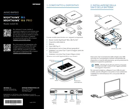
Per caricare la batteria, collegare il cavo USB al router mobile, quindi collegarlo a una presa a muro utilizzando l'adattatore di alimentazione CA o una porta USB del computer.Assicurarsi che l'orientamento della scheda nano SIM coincida con l'orientamento indicato sull'etichetta del dispositivo e inserirla delicatamente, quindi posizionare la batteria e il coperchio posteriore.NOTA: utilizzare solo le dita per inserire o rimuovere la scheda nano SIM. L'utilizzo di altri oggetti potrebbe danneggiare il dispositivo.1. COM'È FATTO IL DISPOSITIVO2. INSTALLAZIONE DELLA SIM E DELLA BATTERIAIl router mobile viene fornito con i seguenti componenti:• Router mobile Nighthawk® M6 o M6 Pro 5G*• Coperchio della batteria • Batteria• Cavo USB Tipo C• Alimentatore (varia in base all’area geografica)• Adattatori con presa Tipo C (per la maggior parte dei Paesi europei)•Adattatori con presa Tipo G (per il Regno Unito)*Illustrazioni del modello Nighthawk M6 per scopi illustrativi.antenna esterna (TS-9)antenna esterna (TS-9)USB Tipo CEthernetCONFORMITÀ NORMATIVA E NOTE LEGALIPer informazioni sulla conformità alle normative, compresala Dichiarazione di conformità UE, visitare il sito Web https:///it/about/regulatory/.Prima di collegare l'alimentazione, consultare il documento relativo alla conformità normativa.Può essere applicato solo ai dispositivi da 6 GHz: utilizzare il dispositivo solo in un ambiente al chiuso. L'utilizzo di dispositivi a 6 GHz è vietato su piattaforme petrolifere, automobili, treni, barche e aerei, tuttavia il suo utilizzo è consentito su aerei di grandi dimensioni quando volano sopra i 3000 metri di altezza. L'utilizzo di trasmettitori nella banda 5.925‑7.125 GHz è vietato per il controllo o le comunicazioni con sistemi aerei senza equipaggio.SUPPORTO E COMMUNITYDalla pagina del portale di amministrazione Web, fare clic sull'icona con i tre puntini nell'angolo in alto a destra per accedere ai file della guida e del supporto.Per ulteriori informazioni, visitare il sito netgear.it/support per accedere al manuale dell'utente completo e per scaricare gli aggiornamenti del firmware.È possibile trovare utili consigli anche nella Community NETGEAR, alla pagina /it.GESTIONE DELLE IMPOSTAZIONI TRAMITE L'APP NETGEAR MOBILEUtilizzare l'app NETGEAR Mobile per modificare il nome della rete Wi-Fi e la password. È possibile utilizzarla anche per riprodurre e condividere contenutimultimediali e accedere alle funzioni avanzate del router mobile.1. Accertarsi che il dispositivo mobile sia connesso a Internet.2. Eseguire la scansione del codice QR per scaricare l'appNETGEAR Mobile.Connessione con il nome e la password della rete Wi-Fi 1. Aprire il programma di gestione della rete Wi‑Fi deldispositivo.2. Individuare il nome della rete Wi‑Fi del router mobile(NTGR_XXXX) e stabilire una connessione.3. Only Connessione tramite EthernetPer prolungare la durata della batteria, l'opzione Ethernet è disattivata per impostazione predefinita. Per attivarla, toccare Power Manager (Risparmio energia) e passare a Performance Mode (Modalità performance).4. CONNESSIONE A INTERNETÈ possibile connettersi a Internet utilizzando il codice QR del router mobile da uno smartphone oppure selezionando manualmente il nome della rete Wi‑Fi del router e immettendo la password.Connessione tramite codice QR da uno smartphone 1. Toccare l'icona del codice QR sulla schermata inizialedello schermo LCD del router mobile.NOTA: quando è inattivo, lo schermo touch si oscura per risparmiare energia. Premere brevemente e rilasciare il pulsante di alimentazione per riattivare lo schermo.3. CONFIGURAZIONE DEL ROUTER MOBILETenere premuto il pulsante di accensione per due secondi, quindi seguire le istruzioni visualizzate sullo schermo per impostare un nome per la rete Wi‑Fi e una password univoci.La personalizzazione delle impostazioni Wi‑Fi consente di proteggere la rete Wi‑Fi del router mobile.Impostazioni APNIl router mobile legge i dati dalla scheda SIM e determina automaticamente le impostazioni APN (Access Point Name) corrette con i piani dati della maggior parte degli operatori. Tuttavia, se si utilizza un router mobile sbloccato con un operatore o un piano meno comune, potrebbe essere necessario immettere manualmente le impostazioni APN.Se viene visualizzata la schermata APN Setup Required (Configurazione APN richiesta), i dati APN dell’operatore non sono presenti nel nostro database ed è necessario inserirli manualmente. Immettere i valori fornitidall’operatore nei campi corrispondenti, quindi toccare Save (Salva) per completare la configurazione.NOTA: l’operatore determina le proprie informazioni APN e deve fornire le informazioni per il proprio piano dati. Si consiglia di contattare il proprio operatore per le impostazioni APN corrette e di utilizzare solo l’APN suggerito per il piano specifico.Schermata inizialeAl termine della configurazione, il router visualizza la schermata iniziale:Wi‑FiPotenza Carica Rete Codice QR connessione rapida Wi‑FiNome e Wi‑FiIcona del codice QR。

圭堡医堂羞堂麓嶷盘查垫塑生！！魍整！§盎筮！塑￡ｂ虹ＬＭ趟△！！！ｂ坠鱼§璎￡！！Ｑ￡！Ｑ鲢１２塑２：ＹＱｌ：；§：艘２：§欧洲标准变应原联合化妆品筛选变应原对女性面部皮炎患者的斑贴试验周成霞李械李利【摘要ｌ蹦的采矮蚊溯标准嶷辙鳆联合化妆赫筛遴燮应原对女性ｌｌｌｉ鄙发炎患者进行斑贴试验，薅壹主要致竣藤；方法霹弱诊女瞧露帮安炎患者果弼讫绶曩蘩选变绽琢联合黢鞘标灌变应蘸送行褒雅试验，按嚣繇接魅建皮炎瓣究组捶荐标准巅潦缝祭。

结果４ｉ灏焱褴患者逢幸亍了３８静德妆酷筛选变虑原和２６种欧洲标准变腹原的斑贴试验。

熊巾阳性率最高ｆｆ缸他妆鼎筛选变应原计裔鸟洛托品（１２．２０％）、硫柳汞（９．７６％）、双咪唑烷基脲（７．３２％）及ＤＭＤＭ海因（７．３２％），阳性率躐高的欧洲标准嶷成原汁有硫酸镍（２２．２０％）、甲醛（１４．６３％）、对苯二胺（９．７６％）及香料混骨芍势ｆ９。

弱％）。

绥谂辘臻耱，争鏊、岛渗托瑟、骧秘汞、对答：藏、蚕辫浸合耢，双曝迹靛基骣，ＤＭＤＭ海毽等是女瞧嚣零瘦灸患毒主要簸被骧。

【关键词ｌ欧渊标准变琏原；化妆品筛选变赢愿＃巅部皮炎；疆髂试簸ＰａｔｃｈｔｅｓｔｉｎｇｆｏｒｓｅｌｅｃｔｉｏｎｏｆｃｏｓｍｅｔｉｃａｌｌｌｅｒｇｅｎｓｉｎｆｅｍａｌｅｆａｅｉａｌｄｅｒｍａｔｉｔｉｓｂｙＥｕｒｏｐｅａｎｓｔａｎｄａｒｄｏｆｃ０８ｍｍｅｔｉｃａｌｌｅｒｇｅｎｓｚＨ（彤Ｃｈｅｎｇ－ｘｉａ，Ｌ｛ｗ武，乙ｉＬｉ．ＤｅｐａｒｔｍｅｎｔｏｆＤｅｒｍａｔｏｌｏｇｙ，Ｗｅ啦ＣｈｉｎａＨｏｓ“ｐｉｔａｔ，Ｓｉ商＃口镕汝ｉｖｅｒＭｔＹ，酝ｏｎｇｄｕ§１００４１，Ｃｈｉｎａ［Ａｂｓｔｒａｃｔ］ＯｂｊｅｃｔｉｖｅＴｏｉｄｅｎｔｉｆｙｔｈｅｅｏｍｎｑｏｎａｌｌｅｒｇｅｎｓｏｆｔｈｅｆｅｍａｌｅｐａｔｉｅｎｔｓｗｋｈｆａｅｉａｉｄｅｆ—ｍａｔｉｔｉｓｗｉｔｈＥｕｒｏｐｅａｎｓｔａｎｄａｒｄｏｆｃｏｓｍｅｔｉｃａｌｌｅｒｇｅｎｓ．ＭｅｔｈｏｄｓＦｅｍａｌｅｐａｔｉｅｎｔｓｗｉｔｈｆａｃｉａｉｄｅｒｍａｔｉｔｉｓｗｅｒｅｔｅｓｔｅｄｗｉｔｈＥｕｒｏｐｅａｎｓｔａｎｄａｒｄｏｆｃｏｓｍｅｔｉｃａｌｌｅｒｇｅｎｓ．ＴｈｅｒｅａｃｔｉｏｎｓｔｏａｌｌｅｒｇｅｎｓｗｅｒｅｄｏｃｕｍｅｎｔｅｄｈｙｆｏｌｌｏｗｉｎｇｔｈｅＩｎｔｅｒｎａｔｉｏｎａｌＣｏｎｔａｅｔＤｅｒｍａｔｉｔｉｓＲｅｓｅａｒｃｈＧｒｏｕｐｒｅｃｏｍｍｅｎｄａｔｉｏｎｓ．ＲｅｓｕｌｔｓＴｏｔａｌ４ｌｆｅｍａｌｅｐａｔｉｅｎｔｓｗｉｔｈｆａｃｉａｌｄｅｒｍａｔｉｔｉｓｗｅｒｅｔｅｓｔｅｄｗｉｔｈＥｕｒｏｐｅａｎｓｔａｎｄａｒｄｏｆｃｏｓｍｅｔｉｃａｌｌｅｒｇｅｎｓ，ｔｈｅｍａｉｎｃｏｓｍｅｔｉｃａｌｌｅｒｇｅｎｓｖｃｅｒｅｈｅｘａｍｉｎｅ（１２，２０），ｔｈｉｍｅｒｏｓａｌ（９。

DIRECTIVE NUMBER: CPL 02-00-150 EFFECTIVE DATE: April 22, 2011 SUBJECT: Field Operations Manual (FOM)ABSTRACTPurpose: This instruction cancels and replaces OSHA Instruction CPL 02-00-148,Field Operations Manual (FOM), issued November 9, 2009, whichreplaced the September 26, 1994 Instruction that implemented the FieldInspection Reference Manual (FIRM). The FOM is a revision of OSHA’senforcement policies and procedures manual that provides the field officesa reference document for identifying the responsibilities associated withthe majority of their inspection duties. This Instruction also cancels OSHAInstruction FAP 01-00-003 Federal Agency Safety and Health Programs,May 17, 1996 and Chapter 13 of OSHA Instruction CPL 02-00-045,Revised Field Operations Manual, June 15, 1989.Scope: OSHA-wide.References: Title 29 Code of Federal Regulations §1903.6, Advance Notice ofInspections; 29 Code of Federal Regulations §1903.14, Policy RegardingEmployee Rescue Activities; 29 Code of Federal Regulations §1903.19,Abatement Verification; 29 Code of Federal Regulations §1904.39,Reporting Fatalities and Multiple Hospitalizations to OSHA; and Housingfor Agricultural Workers: Final Rule, Federal Register, March 4, 1980 (45FR 14180).Cancellations: OSHA Instruction CPL 02-00-148, Field Operations Manual, November9, 2009.OSHA Instruction FAP 01-00-003, Federal Agency Safety and HealthPrograms, May 17, 1996.Chapter 13 of OSHA Instruction CPL 02-00-045, Revised FieldOperations Manual, June 15, 1989.State Impact: Notice of Intent and Adoption required. See paragraph VI.Action Offices: National, Regional, and Area OfficesOriginating Office: Directorate of Enforcement Programs Contact: Directorate of Enforcement ProgramsOffice of General Industry Enforcement200 Constitution Avenue, NW, N3 119Washington, DC 20210202-693-1850By and Under the Authority ofDavid Michaels, PhD, MPHAssistant SecretaryExecutive SummaryThis instruction cancels and replaces OSHA Instruction CPL 02-00-148, Field Operations Manual (FOM), issued November 9, 2009. The one remaining part of the prior Field Operations Manual, the chapter on Disclosure, will be added at a later date. This Instruction also cancels OSHA Instruction FAP 01-00-003 Federal Agency Safety and Health Programs, May 17, 1996 and Chapter 13 of OSHA Instruction CPL 02-00-045, Revised Field Operations Manual, June 15, 1989. This Instruction constitutes OSHA’s general enforcement policies and procedures manual for use by the field offices in conducting inspections, issuing citations and proposing penalties.Significant Changes∙A new Table of Contents for the entire FOM is added.∙ A new References section for the entire FOM is added∙ A new Cancellations section for the entire FOM is added.∙Adds a Maritime Industry Sector to Section III of Chapter 10, Industry Sectors.∙Revises sections referring to the Enhanced Enforcement Program (EEP) replacing the information with the Severe Violator Enforcement Program (SVEP).∙Adds Chapter 13, Federal Agency Field Activities.∙Cancels OSHA Instruction FAP 01-00-003, Federal Agency Safety and Health Programs, May 17, 1996.DisclaimerThis manual is intended to provide instruction regarding some of the internal operations of the Occupational Safety and Health Administration (OSHA), and is solely for the benefit of the Government. No duties, rights, or benefits, substantive or procedural, are created or implied by this manual. The contents of this manual are not enforceable by any person or entity against the Department of Labor or the United States. Statements which reflect current Occupational Safety and Health Review Commission or court precedents do not necessarily indicate acquiescence with those precedents.Table of ContentsCHAPTER 1INTRODUCTIONI.PURPOSE. ........................................................................................................... 1-1 II.SCOPE. ................................................................................................................ 1-1 III.REFERENCES .................................................................................................... 1-1 IV.CANCELLATIONS............................................................................................. 1-8 V. ACTION INFORMATION ................................................................................. 1-8A.R ESPONSIBLE O FFICE.......................................................................................................................................... 1-8B.A CTION O FFICES. .................................................................................................................... 1-8C. I NFORMATION O FFICES............................................................................................................ 1-8 VI. STATE IMPACT. ................................................................................................ 1-8 VII.SIGNIFICANT CHANGES. ............................................................................... 1-9 VIII.BACKGROUND. ................................................................................................. 1-9 IX. DEFINITIONS AND TERMINOLOGY. ........................................................ 1-10A.T HE A CT................................................................................................................................................................. 1-10B. C OMPLIANCE S AFETY AND H EALTH O FFICER (CSHO). ...........................................................1-10B.H E/S HE AND H IS/H ERS ..................................................................................................................................... 1-10C.P ROFESSIONAL J UDGMENT............................................................................................................................... 1-10E. W ORKPLACE AND W ORKSITE ......................................................................................................................... 1-10CHAPTER 2PROGRAM PLANNINGI.INTRODUCTION ............................................................................................... 2-1 II.AREA OFFICE RESPONSIBILITIES. .............................................................. 2-1A.P ROVIDING A SSISTANCE TO S MALL E MPLOYERS. ...................................................................................... 2-1B.A REA O FFICE O UTREACH P ROGRAM. ............................................................................................................. 2-1C. R ESPONDING TO R EQUESTS FOR A SSISTANCE. ............................................................................................ 2-2 III. OSHA COOPERATIVE PROGRAMS OVERVIEW. ...................................... 2-2A.V OLUNTARY P ROTECTION P ROGRAM (VPP). ........................................................................... 2-2B.O NSITE C ONSULTATION P ROGRAM. ................................................................................................................ 2-2C.S TRATEGIC P ARTNERSHIPS................................................................................................................................. 2-3D.A LLIANCE P ROGRAM ........................................................................................................................................... 2-3 IV. ENFORCEMENT PROGRAM SCHEDULING. ................................................ 2-4A.G ENERAL ................................................................................................................................................................. 2-4B.I NSPECTION P RIORITY C RITERIA. ..................................................................................................................... 2-4C.E FFECT OF C ONTEST ............................................................................................................................................ 2-5D.E NFORCEMENT E XEMPTIONS AND L IMITATIONS. ....................................................................................... 2-6E.P REEMPTION BY A NOTHER F EDERAL A GENCY ........................................................................................... 2-6F.U NITED S TATES P OSTAL S ERVICE. .................................................................................................................. 2-7G.H OME-B ASED W ORKSITES. ................................................................................................................................ 2-8H.I NSPECTION/I NVESTIGATION T YPES. ............................................................................................................... 2-8 V.UNPROGRAMMED ACTIVITY – HAZARD EVALUATION AND INSPECTION SCHEDULING ............................................................................ 2-9 VI.PROGRAMMED INSPECTIONS. ................................................................... 2-10A.S ITE-S PECIFIC T ARGETING (SST) P ROGRAM. ............................................................................................. 2-10B.S CHEDULING FOR C ONSTRUCTION I NSPECTIONS. ..................................................................................... 2-10C.S CHEDULING FOR M ARITIME I NSPECTIONS. ............................................................................. 2-11D.S PECIAL E MPHASIS P ROGRAMS (SEP S). ................................................................................... 2-12E.N ATIONAL E MPHASIS P ROGRAMS (NEP S) ............................................................................... 2-13F.L OCAL E MPHASIS P ROGRAMS (LEP S) AND R EGIONAL E MPHASIS P ROGRAMS (REP S) ............ 2-13G.O THER S PECIAL P ROGRAMS. ............................................................................................................................ 2-13H.I NSPECTION S CHEDULING AND I NTERFACE WITH C OOPERATIVE P ROGRAM P ARTICIPANTS ....... 2-13CHAPTER 3INSPECTION PROCEDURESI.INSPECTION PREPARATION. .......................................................................... 3-1 II.INSPECTION PLANNING. .................................................................................. 3-1A.R EVIEW OF I NSPECTION H ISTORY .................................................................................................................... 3-1B.R EVIEW OF C OOPERATIVE P ROGRAM P ARTICIPATION .............................................................................. 3-1C.OSHA D ATA I NITIATIVE (ODI) D ATA R EVIEW .......................................................................................... 3-2D.S AFETY AND H EALTH I SSUES R ELATING TO CSHO S.................................................................. 3-2E.A DVANCE N OTICE. ................................................................................................................................................ 3-3F.P RE-I NSPECTION C OMPULSORY P ROCESS ...................................................................................................... 3-5G.P ERSONAL S ECURITY C LEARANCE. ................................................................................................................. 3-5H.E XPERT A SSISTANCE. ........................................................................................................................................... 3-5 III. INSPECTION SCOPE. ......................................................................................... 3-6A.C OMPREHENSIVE ................................................................................................................................................... 3-6B.P ARTIAL. ................................................................................................................................................................... 3-6 IV. CONDUCT OF INSPECTION .............................................................................. 3-6A.T IME OF I NSPECTION............................................................................................................................................. 3-6B.P RESENTING C REDENTIALS. ............................................................................................................................... 3-6C.R EFUSAL TO P ERMIT I NSPECTION AND I NTERFERENCE ............................................................................. 3-7D.E MPLOYEE P ARTICIPATION. ............................................................................................................................... 3-9E.R ELEASE FOR E NTRY ............................................................................................................................................ 3-9F.B ANKRUPT OR O UT OF B USINESS. .................................................................................................................... 3-9G.E MPLOYEE R ESPONSIBILITIES. ................................................................................................. 3-10H.S TRIKE OR L ABOR D ISPUTE ............................................................................................................................. 3-10I. V ARIANCES. .......................................................................................................................................................... 3-11 V. OPENING CONFERENCE. ................................................................................ 3-11A.G ENERAL ................................................................................................................................................................ 3-11B.R EVIEW OF A PPROPRIATION A CT E XEMPTIONS AND L IMITATION. ..................................................... 3-13C.R EVIEW S CREENING FOR P ROCESS S AFETY M ANAGEMENT (PSM) C OVERAGE............................. 3-13D.R EVIEW OF V OLUNTARY C OMPLIANCE P ROGRAMS. ................................................................................ 3-14E.D ISRUPTIVE C ONDUCT. ...................................................................................................................................... 3-15F.C LASSIFIED A REAS ............................................................................................................................................. 3-16VI. REVIEW OF RECORDS. ................................................................................... 3-16A.I NJURY AND I LLNESS R ECORDS...................................................................................................................... 3-16B.R ECORDING C RITERIA. ...................................................................................................................................... 3-18C. R ECORDKEEPING D EFICIENCIES. .................................................................................................................. 3-18 VII. WALKAROUND INSPECTION. ....................................................................... 3-19A.W ALKAROUND R EPRESENTATIVES ............................................................................................................... 3-19B.E VALUATION OF S AFETY AND H EALTH M ANAGEMENT S YSTEM. ....................................................... 3-20C.R ECORD A LL F ACTS P ERTINENT TO A V IOLATION. ................................................................................. 3-20D.T ESTIFYING IN H EARINGS ................................................................................................................................ 3-21E.T RADE S ECRETS. ................................................................................................................................................. 3-21F.C OLLECTING S AMPLES. ..................................................................................................................................... 3-22G.P HOTOGRAPHS AND V IDEOTAPES.................................................................................................................. 3-22H.V IOLATIONS OF O THER L AWS. ....................................................................................................................... 3-23I.I NTERVIEWS OF N ON-M ANAGERIAL E MPLOYEES .................................................................................... 3-23J.M ULTI-E MPLOYER W ORKSITES ..................................................................................................................... 3-27 K.A DMINISTRATIVE S UBPOENA.......................................................................................................................... 3-27 L.E MPLOYER A BATEMENT A SSISTANCE. ........................................................................................................ 3-27 VIII. CLOSING CONFERENCE. .............................................................................. 3-28A.P ARTICIPANTS. ..................................................................................................................................................... 3-28B.D ISCUSSION I TEMS. ............................................................................................................................................ 3-28C.A DVICE TO A TTENDEES .................................................................................................................................... 3-29D.P ENALTIES............................................................................................................................................................. 3-30E.F EASIBLE A DMINISTRATIVE, W ORK P RACTICE AND E NGINEERING C ONTROLS. ............................ 3-30F.R EDUCING E MPLOYEE E XPOSURE. ................................................................................................................ 3-32G.A BATEMENT V ERIFICATION. ........................................................................................................................... 3-32H.E MPLOYEE D ISCRIMINATION .......................................................................................................................... 3-33 IX. SPECIAL INSPECTION PROCEDURES. ...................................................... 3-33A.F OLLOW-UP AND M ONITORING I NSPECTIONS............................................................................................ 3-33B.C ONSTRUCTION I NSPECTIONS ......................................................................................................................... 3-34C. F EDERAL A GENCY I NSPECTIONS. ................................................................................................................. 3-35CHAPTER 4VIOLATIONSI. BASIS OF VIOLATIONS ..................................................................................... 4-1A.S TANDARDS AND R EGULATIONS. .................................................................................................................... 4-1B.E MPLOYEE E XPOSURE. ........................................................................................................................................ 4-3C.R EGULATORY R EQUIREMENTS. ........................................................................................................................ 4-6D.H AZARD C OMMUNICATION. .............................................................................................................................. 4-6E. E MPLOYER/E MPLOYEE R ESPONSIBILITIES ................................................................................................... 4-6 II. SERIOUS VIOLATIONS. .................................................................................... 4-8A.S ECTION 17(K). ......................................................................................................................... 4-8B.E STABLISHING S ERIOUS V IOLATIONS ............................................................................................................ 4-8C. F OUR S TEPS TO BE D OCUMENTED. ................................................................................................................... 4-8 III. GENERAL DUTY REQUIREMENTS ............................................................. 4-14A.E VALUATION OF G ENERAL D UTY R EQUIREMENTS ................................................................................. 4-14B.E LEMENTS OF A G ENERAL D UTY R EQUIREMENT V IOLATION.............................................................. 4-14C. U SE OF THE G ENERAL D UTY C LAUSE ........................................................................................................ 4-23D.L IMITATIONS OF U SE OF THE G ENERAL D UTY C LAUSE. ..............................................................E.C LASSIFICATION OF V IOLATIONS C ITED U NDER THE G ENERAL D UTY C LAUSE. ..................F. P ROCEDURES FOR I MPLEMENTATION OF S ECTION 5(A)(1) E NFORCEMENT ............................ 4-25 4-27 4-27IV.OTHER-THAN-SERIOUS VIOLATIONS ............................................... 4-28 V.WILLFUL VIOLATIONS. ......................................................................... 4-28A.I NTENTIONAL D ISREGARD V IOLATIONS. ..........................................................................................4-28B.P LAIN I NDIFFERENCE V IOLATIONS. ...................................................................................................4-29 VI. CRIMINAL/WILLFUL VIOLATIONS. ................................................... 4-30A.A REA D IRECTOR C OORDINATION ....................................................................................................... 4-31B.C RITERIA FOR I NVESTIGATING P OSSIBLE C RIMINAL/W ILLFUL V IOLATIONS ........................ 4-31C. W ILLFUL V IOLATIONS R ELATED TO A F ATALITY .......................................................................... 4-32 VII. REPEATED VIOLATIONS. ...................................................................... 4-32A.F EDERAL AND S TATE P LAN V IOLATIONS. ........................................................................................4-32B.I DENTICAL S TANDARDS. .......................................................................................................................4-32C.D IFFERENT S TANDARDS. .......................................................................................................................4-33D.O BTAINING I NSPECTION H ISTORY. .....................................................................................................4-33E.T IME L IMITATIONS..................................................................................................................................4-34F.R EPEATED V. F AILURE TO A BATE....................................................................................................... 4-34G. A REA D IRECTOR R ESPONSIBILITIES. .............................................................................. 4-35 VIII. DE MINIMIS CONDITIONS. ................................................................... 4-36A.C RITERIA ................................................................................................................................................... 4-36B.P ROFESSIONAL J UDGMENT. ..................................................................................................................4-37C. A REA D IRECTOR R ESPONSIBILITIES. .............................................................................. 4-37 IX. CITING IN THE ALTERNATIVE ............................................................ 4-37 X. COMBINING AND GROUPING VIOLATIONS. ................................... 4-37A.C OMBINING. ..............................................................................................................................................4-37B.G ROUPING. ................................................................................................................................................4-38C. W HEN N OT TO G ROUP OR C OMBINE. ................................................................................................4-38 XI. HEALTH STANDARD VIOLATIONS ....................................................... 4-39A.C ITATION OF V ENTILATION S TANDARDS ......................................................................................... 4-39B.V IOLATIONS OF THE N OISE S TANDARD. ...........................................................................................4-40 XII. VIOLATIONS OF THE RESPIRATORY PROTECTION STANDARD(§1910.134). ....................................................................................................... XIII. VIOLATIONS OF AIR CONTAMINANT STANDARDS (§1910.1000) ... 4-43 4-43A.R EQUIREMENTS UNDER THE STANDARD: .................................................................................................. 4-43B.C LASSIFICATION OF V IOLATIONS OF A IR C ONTAMINANT S TANDARDS. ......................................... 4-43 XIV. CITING IMPROPER PERSONAL HYGIENE PRACTICES. ................... 4-45A.I NGESTION H AZARDS. .................................................................................................................................... 4-45B.A BSORPTION H AZARDS. ................................................................................................................................ 4-46C.W IPE S AMPLING. ............................................................................................................................................. 4-46D.C ITATION P OLICY ............................................................................................................................................ 4-46 XV. BIOLOGICAL MONITORING. ...................................................................... 4-47CHAPTER 5CASE FILE PREPARATION AND DOCUMENTATIONI.INTRODUCTION ............................................................................................... 5-1 II.INSPECTION CONDUCTED, CITATIONS BEING ISSUED. .................... 5-1A.OSHA-1 ................................................................................................................................... 5-1B.OSHA-1A. ............................................................................................................................... 5-1C. OSHA-1B. ................................................................................................................................ 5-2 III.INSPECTION CONDUCTED BUT NO CITATIONS ISSUED .................... 5-5 IV.NO INSPECTION ............................................................................................... 5-5 V. HEALTH INSPECTIONS. ................................................................................. 5-6A.D OCUMENT P OTENTIAL E XPOSURE. ............................................................................................................... 5-6B.E MPLOYER’S O CCUPATIONAL S AFETY AND H EALTH S YSTEM. ............................................................. 5-6 VI. AFFIRMATIVE DEFENSES............................................................................. 5-8A.B URDEN OF P ROOF. .............................................................................................................................................. 5-8B.E XPLANATIONS. ..................................................................................................................................................... 5-8 VII. INTERVIEW STATEMENTS. ........................................................................ 5-10A.G ENERALLY. ......................................................................................................................................................... 5-10B.CSHO S SHALL OBTAIN WRITTEN STATEMENTS WHEN: .......................................................................... 5-10C.L ANGUAGE AND W ORDING OF S TATEMENT. ............................................................................................. 5-11D.R EFUSAL TO S IGN S TATEMENT ...................................................................................................................... 5-11E.V IDEO AND A UDIOTAPED S TATEMENTS. ..................................................................................................... 5-11F.A DMINISTRATIVE D EPOSITIONS. .............................................................................................5-11 VIII. PAPERWORK AND WRITTEN PROGRAM REQUIREMENTS. .......... 5-12 IX.GUIDELINES FOR CASE FILE DOCUMENTATION FOR USE WITH VIDEOTAPES AND AUDIOTAPES .............................................................. 5-12 X.CASE FILE ACTIVITY DIARY SHEET. ..................................................... 5-12 XI. CITATIONS. ..................................................................................................... 5-12A.S TATUTE OF L IMITATIONS. .............................................................................................................................. 5-13B.I SSUING C ITATIONS. ........................................................................................................................................... 5-13C.A MENDING/W ITHDRAWING C ITATIONS AND N OTIFICATION OF P ENALTIES. .................................. 5-13D.P ROCEDURES FOR A MENDING OR W ITHDRAWING C ITATIONS ............................................................ 5-14 XII. INSPECTION RECORDS. ............................................................................... 5-15A.G ENERALLY. ......................................................................................................................................................... 5-15B.R ELEASE OF I NSPECTION I NFORMATION ..................................................................................................... 5-15C. C LASSIFIED AND T RADE S ECRET I NFORMATION ...................................................................................... 5-16。