Comparison of TSP Algorithms(2-OPT,3-OPT)
- 格式:pdf
- 大小:225.37 KB
- 文档页数:21

TSP问题的几种常用求解算法比较旅行商问题(Traveling Salesman Problem, TSP)是典型的组合优化问题,很多优化问题都可以直接或间接的转为为TSP问题,而且TSP问题已被证明具有NPC计算复杂性,有很大的求解难度,因此研究TSP问题的求解方法有着很大的实际意义。
本文旨在介绍求解TSP的几种常用解法,并结合实例比较这些算法的性能,为TSP的求解提供一些参考。
1 TSP问题描述TSP问题的数学表述为:一个有穷的城市集合C={C1,C2,…,Cm},对于每一对城市Ci,Cj∈C有距离d(Ci,Cj)∈R+。
问:经过C中所有城市的旅行路线,记为序列,是否存在最小的正数B,对所有可能的序列都有2 TSP问题几种常用求解方法TSP问题有着很多求解算法,主要有。
2.1 贪婪算法贪婪算法[2](Greedy algorithm)是求解大规模TSP问题的常用算法之一,是一种求解优化问题的简单、迅速的求解办法。
贪婪法有限考虑当前情况下最优的优化测度,自顶向下,逐步迭代,具有算法简单,耗时短的特点。
但贪婪算法的求解结果往往不是最优的,甚至可能与全局最优解间有不小的差距。
2.2 模拟退火算法模拟退火(Simulated Annealing,SA)算法是求解TSP问题的有效方法之一,容易编程实现,求解速度快。
模拟退火是一种全局优化算法,加入了随机状态模型,使算法以概率选择的方式逼近最优状态,其收敛性可以得到严格的理论证明。
模拟退火算法具有一整套完整的退火搜索计划,包括足够高的初始温度、缓慢的退火速度、大量的迭代次数及足够的概率扰动[3]。
2.3 遗传算法遗传算法(Genetic Algorithm,GA)是一种常用的智能算法,具有全局搜索能力,对TSP问题有良好的效果。
遗传算法是由Michigan大学的J.Holland教授于1975年提出,算法通常由编码、个体适应度评估和遗传运算三部分构成,其中遗传运算包括染色体复制、交叉、变异和倒位等[4]。
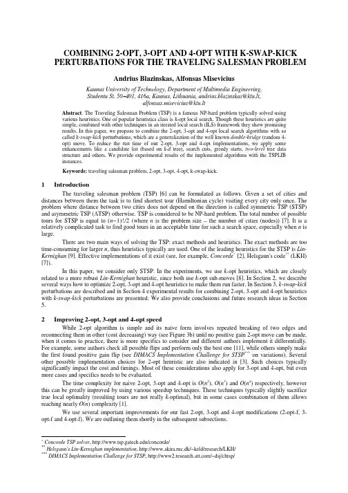
COMBINING 2-OPT, 3-OPT AND 4-OPT WITH K-SWAP-KICK PERTURBATIONS FOR THE TRAVELING SALESMAN PROBLEMAndrius Blazinskas, Alfonsas MiseviciusKaunas University of Technology, Department of Multimedia Engineering,Studentu St. 50−401, 416a, Kaunas, Lithuania, andrius.blazinskas@ktu.lt,alfonsas.misevicius@ktu.ltAbstract. The Traveling Salesman Problem (TSP) is a famous NP-hard problem typically solved usingvarious heuristics. One of popular heuristics class is k-opt local search. Though these heuristics are quitesimple, combined with other techniques in an iterated local search (ILS) framework they show promisingresults. In this paper, we propose to combine the 2-opt, 3-opt and 4-opt local search algorithms with socalled k-swap-kick perturbations, which are a generalization of the well known double-bridge (random 4-opt) move. To reduce the run time of our 2-opt, 3-opt and 4-opt implementations, we apply someenhancements like a candidate list (based on k-d tree), search cuts, greedy starts, two-level tree datastructure and others. We provide experimental results of the implemented algorithms with the TSPLIBinstances.Keywords: traveling salesman problem, 2-opt, 3-opt, 4-opt, k-swap-kick.1IntroductionThe traveling salesman problem (TSP) [6] can be formulated as follows. Given a set of cities and distances between them the task is to find shortest tour (Hamiltonian cycle) visiting every city only once. The problem where distance between two cities does not depend on the direction is called symmetric TSP (STSP) and asymmetric TSP (ATSP) otherwise. TSP is considered to be NP-hard problem. The total number of possible tours for STSP is equal to (n−1)!/2 (where n is the problem size – the number of cities (nodes)) [7]. It is a relatively complicated task to find good tours in an acceptable time for such a search space, especially when n is large.There are two main ways of solving the TSP: exact methods and heuristics. The exact methods are too time-consuming for larger n, thus heuristics typically are used. One of the leading heuristics for the STSP is Lin-Kernighan [9]. Effective implementations of it exist (see, for example, Concorde* [2], Helsgaun's code** (LKH) [7]).In this paper, we consider only STSP. In the experiments, we use k-opt heuristics, which are closely related to a more robust Lin-Kernighan heuristic, since both use k-opt sub-moves [8]. In Section 2, we describe several ways how to optimize 2-opt, 3-opt and 4-opt heuristics to make them run faster. In Section 3, k-swap-kick perturbations are described and in Section 4 experimental results for combining 2-opt, 3-opt and 4-opt heuristics with k-swap-kick perturbations are presented. We also provide conclusions and future research ideas in Section 5.2Improving 2-opt, 3-opt and 4-opt speedWhile 2-opt algorithm is simple and its naive form involves repeated breaking of two edges and reconnecting them in other (cost decreasing) way (see Figure 3b) until no positive gain 2-opt move can be made, when it comes to practice, there is more specifics to consider and different authors implement it differentially. For example, some authors check all possible flips and perform only the best one [11], while others simply make the first found positive gain flip (see DIMACS Implementation Challenge for STSP***on variations). Several other possible implementation choices for 2-opt heuristic are also indicated in [3]. Such choices typically significantly impact the cost and timings. Most of these considerations also apply for 3-opt and 4-opt, but even more cases and specifics needs to be evaluated.The time complexity for naive 2-opt, 3-opt and 4-opt is O(n2), O(n3) and O(n4) respectively, however this can be greatly improved by using various speedup techniques. These techniques typically slightly sacrifice true local optimality (resulting tours are not really k-optimal), but in some cases combination of them allows reaching nearly O(n) complexity [1].We use several important improvements for our fast 2-opt, 3-opt and 4-opt modifications (2-opt-f, 3-opt-f and 4-opt-f). We are outlining them shortly in the subsequent subsections.*Concorde TSP solver, /concorde/**Helsgaun's Lin-Kernighan implementation, http://www.akira.ruc.dk/~keld/research/LKH/***DIMACS Implementation Challenge for STSP, /~dsj/chtsp/2.1K-d tree based candidate listNearest node candidate lists (CL) are widely used for improving k-opt heuristics [1]. K-d tree usage for CL identification is much more efficient than naive CL approach. In particular, naive CL can be generated in O(n2log n) time [11], while k-d tree − in O(Kn + n log n) [4] (where K is the number of dimensions and in our case always K = 2). Once generated, naive CL does not require any additional processing to extract lists (it simply contains them in arrays), while k-d tree needs to be searched every time a list is needed. This, of course, can be solved by using caching, but for large TSP instances caching requires a lot of memory which grows in O(mn) (where m– CL size) and for storing k-d tree this number is roughly O(n) (efficient Concorde k-d tree implementation uses 52n bytes of memory). Searching in k-d tree (bottom-up technique) can be done in almost O(1) time [4]. Thus efficient k-d tree implementation beats naive CL practically in all cases. Benefits of using k-d tree for CL are obvious, for example, on our test machine (see Section 4 for specifications) for pla85900 TSP problem instance construction of CL in naive way takes roughly 15 minutes, while construction of k-d tree with searching and caching of CL – about 3 seconds (CL size in both cases is equal to 80). It must be noted, that usage of k-d tree limits TSP solver to Euclidean instances.2.2Stop search if b1 = a2Instead of a popular don't look bits idea [1], we propose using search cut if a1 nearest candidate b1 is already the next node to a1 (that is, a2 = b1) in the current tour (see Figure 2 for pseudo code). A similar cut is used for 2-opt fixed-radius search in [3]. We also use such cuts for 3-opt and 4-opt when b2 = c1 and c2 = d1. Our experiments indicate that these improvements greatly shorten running times without significantly increasing cost.2.3For 3-opt and 4-opt consider cases where only 3 and 4 edges are exchanged respectivelyWhile breaking k edges in a tour, there are (k−1)!2k−1 ways to reconnect it (including the initial tour) to form a valid tour [6], typically not all of these cases are considered [15]. In our implementation, we consider only those cases where all k edges are new. For example, breaking 3 edges in 3-opt there are in total 8 cases for reconnection (Figure 1), but only 4 of them (e, f, g, h) actually introduce all new edges (all others, except initial one, are simple 2-opt moves). Similarly for 4-opt, breaking 4 edges we have 48 ways to reconnect, but only 25 cases offer all 4 new edges. This does not affect 2-opt heuristic, since there is only one way to reconnect to a valid tour.Figure 1. All possible 3-opt reconnection cases2.4Cascading 3-opt and 4-optWe have noticed that cascading k-opt heuristics reduces overall running time. We exploit this feature in this way: for 3-opt-f, we additionally preprocess tours with 2-opt-f and for 4-opt-f preprocessing is done with 2-opt-f and 3-opt-f in this order. Optimization is started from random node every time.2.5Greedy multi-fragment initial toursMulti-fragment heuristic (simply called Greedy heuristic) is an effective tour construction heuristic proposed in [3]. It is known to be particularly good as a preprocessor for k-opt heuristics and more effective than traditional nearest-neighbour heuristic [1, 3]. Using such greedy starting tours in k-opt, improvement is observed for both – tour quality and running times. In our implementation, multi-fragment tour construction is backed with earlier described k-d tree for efficiency reasons. Complexity for this heuristic is O(n log n) [3]. It should be noted, that it makes sense to use this heuristic only once for particular problem, since there is no different starting points like with the nearest-neighbor and thus the resulting tour is always the same.2.6Two-level tree data structureTwo-level tree [5] is one of the most popular data structures for tour representation in the TSP [1, 7]. It offers O(√ܰ) complexity for reversing (flipping) the sub-tour – one of the most common operations in the TSP. It is useful for problems where n≤ 106, otherwise Splay trees seems to be a better choice [5]. It should be noted, that usage of two-level tree is helpful only within the optimized k-opt heuristics, where time required for flip operation becomes dominant. In our experiments for naive 2-opt, only changing array with two-level tree resulted in higher running times: traversing through nodes in two-level tree is more costly, since it requires accessing parent nodes and performing additional checks (though still O(1), the constant is actually larger), whilefor simple array representation it is on mentioned improvements, a rough pseu procedure fast4Opt (tour , cl , cost localyOptimal := FALSE ;while (not localyOptimal ) localyOptimal := TRU a 1 := startNode ; repeat a 2 := next for (∀b 1 ϵ end enda 1 := next (a until (a 1 == startNode endend fast4OptFigure 2. 3 K-swap-kick perturbation The simplest non-sequential and later recognized as an effective mu in one of the most powerful heuristics kick (a concatenation of k segments LKH considered improving k -opt mov we will be applying k-swap-kicks to will consider all same pattern having k-swap-kicks illustration for k = 3, 4 Figure 3. 2-opt move and k-swap-kick All k-swap-kicks are special c of n ≥ 2k is enough.We will be analyzing only ra effect on tour cost during perturbation in k -opt heuristics, which typically perf Random double-bridge move [1]. In some cases, it even yielded Lin-Kernighan . We continue by extenandis only a matter of increasing or decreasing the array index h pseudo code for the fast 4-opt implementation is provided costs , startNode ) beginbegin TRUE ; (a 1); cl (a 1)) begin if (a 2 == b 1) break ; // speedup b 2 := next (b 1); for (∀c 1 ϵ cl (b 1)) begin if (b 2 == c 1) break ; // speedup c 2 := next (c 1); for (∀d 1 ϵ cl (c 1)) begin if (c 2 == d 1) break ; // speedup d 2 := next (d 1); findBestReconnection (a 1, a 2, b 1, b 2, c 1, if (better reconnection exists) begin reconnect (a 1, a 2, b 1, b 2, c 1, c 2, localyOptimal := false; end end end 1); Node ); . General pseudo code for fast 4-opt implementationonntial k -opt move is a double-bridge move (4-opt move) [8ve mutation operator [10]. It is well known move, random ristics – Iterated Lin-Kernighan [1]. A generalization of th ents: s 1, s k , s k −1,...,s 2) introduced in [14] as an improvemen moves of size k ≤ 5, it was proposed to use k-swap-kicks to our fast 2-opt, 3-opt and 4-opt heuristics, we will omi ving moves with k ≥ 3 and simple 2-opt move (k = 2). Graph 4 is provided in Figure 3.ick perturbations: a) initial tour, b) 2-opt move, c) 3-opt move bridge or 4-opt move (k = 4)cial cases of k -opt moves. Clearly for k-swap-kick to be pe nly random 2-opt and k-swap-kick moves, the ones which ation and may typically lead to worse tours. This is opposi perform only tour-cost-decreasing moves.move previously was also combined with 3-opt heuristic, fo ed better results to that of Lin-Kernighan and was slightlyextending this idea. We perform an experiment combining index. Considering above vided in Figure 2.c 2,d 1, d 2, costs ); d 1, d 2, tour ); 8] first mentioned in [9]ndom version of it is used of this move is a k-swap-vement for LKH. Because kicks of size k ≥ 6. Since l omit this restriction. We Graphical 2-opt move andmove (k=3) and d) double-be performed, a condition which do not consider thepposite to the moves used tic, forming Iterated 3-optightly worse than Iteratedbining our 2-opt-f, 3-opt-f4-opt-f implementations with random 2-opt move and random k-swap-kicks (k = 3...15). Pseudo code on how this combination is implemented is provided in Figure 4b.z * := ∞;repeatGenerate a greedy randomized solution t ;Find local optimum t l with local search starting from t ; if (z(t l ) < z*) begin z* := z(t l ); t* := t l ;enduntil a stopping criterion is satisfied;Generate a greedy solution t ;Find local optimum t l with local search starting from t ; z* := z (t l );repeatPerturb t l tour using random k-swap-kick forming t lp ;Find local optimum t lpl with local search starting from t lp ; if (z(t lpl ) < z*) begin z* := z(t lpl ); t* := t l := t lpl ;enduntil a stopping criterion is satisfied;(a)(b)Figure 4. General pseudo codes for GRASP (a) and k-swap-kick perturbation (b) frameworks (t* – best solution foundand z* = z(t*), where z – objective function)It should be noted that k-swap-kick ILS framework is quite similar to other well known procedure –GRASP (see Figure 4a, also see [12]). The main distinction between them is that GRASP starts from a totally different initial tour in every iteration, rather than perturbing existing one.4 Experimental resultsAll algorithms are fully implemented using Java (JDK 6). Implementations of two-level tree, k-d treeand multi-fragment heuristic are based on Concorde C code . Experiments were performed on the machine with Intel Core i7-860 processor and 8GB of RAM.Below provided tables and graphs summarize the results of our fast 2-opt, 3-opt and 4-optimplementations (2-opt-f, 3-opt-f and 4-opt-f). To emphasize the advantage of perturbations, we also performed two additional experiments without using perturbations: one with random starts and other with greedy starts. In these experiments, we used similar to GRASP procedure, but it did not fully comply with basic GRASP scheme (see Figure 4a): random start experiment did not use greedy randomized heuristic for initial solution and greedy start experiment had no randomization (since we were using original multi-fragment heuristic). The only randomization in later case was different start point (node) in fast k -opt local search. All other consecutive columns provide the results for random 2-opt (k = 2) and k-swap-kick perturbations with fixed k . In both frameworks, the number of iterations was set to 1000 (stopping criterion). Deviations from the optimal tour length (optimal tour lengths can be found in TSPLIB [13]) were estimated using formula: %][ ) *(100opt opt z z z −=δ, where z * – obtained best value of the objective function and z opt denotes the provably optimal objective function value. All experiments were repeated for 10 times and averages calculated. The problem data for experiments were taken from the TSP library – TSPLIB [13].Table 1. Experimental results for 4-opt-f: tour quality (average deviation from optimal of 10 runs, %) Problem name 4-opt-f 4-opt-f with greedy start and k-swap-kicksRandom start Greedy start kBest found(k ) 2 3 4 5 6 10 15 eil51 0.00 1.17 0.02 0.07 0.05 0.02 0.12 0.00 0.02 0 (all) st70 0.00 3.26 0.00 0.00 0.00 0.00 0.00 0.00 0.00 0 (all) kroE100 0.03 0.00 0.00 0.00 0.03 0.02 0.00 0.00 0.02 0 (all) kroB150 0.19 2.11 0.11 0.02 0.04 0.04 0.02 0.03 0.03 0 (all) ts225 0.21 1.35 0.02 0.00 0.00 0.00 0.00 0.00 0.00 0 (all) gil262 1.73 2.11 0.40 0.46 0.13 0.14 0.23 0.20 0.27 0 (4, 6) a280 1.81 1.98 0.64 0.48 0.02 0.05 0.20 0.03 0.04 0 (all) lin318 1.66 2.09 0.54 0.49 0.36 0.42 0.35 0.37 0.54 0 (2, 4) rd400 2.42 2.10 0.57 0.33 0.24 0.33 0.29 0.51 0.54 0.07 (4, 6) u574 2.98 2.50 1.18 0.53 0.62 0.63 0.69 0.79 1.06 0.13 (3) rat783 3.96 2.58 1.43 1.00 1.11 1.13 1.19 1.55 1.78 0.48 (3) vm1084 3.05 1.92 0.87 0.47 0.47 0.60 0.50 0.77 0.98 0.15 (3, 4) pcb1173 4.92 3.78 2.10 1.76 1.45 1.77 1.82 2.15 2.54 1.17 (4) vm1748 3.68 2.89 1.24 0.81 0.85 0.96 1.08 1.23 1.52 0.50 (4) d2103 6.33 2.46 1.20 0.91 0.82 1.22 1.22 1.53 1.80 0.27 (4) fnl4461 4.96 2.57 2.21 2.19 2.17 2.44 2.47 2.76 2.74 1.92 (2) rl59345.712.952.06 1.82 1.81 2.21 2.08 2.693.071.47 (3)Problem name4-opt-f 4-opt-f with greedy start and k-swap-kicksRandom start Greedy start kBest found (k ) 2 3 4 5 6 10 15pla7397 4.85 2.94 2.01 1.74 1.62 2.04 1.86 2.28 2.71 1.34 (4) rl11849 6.30 2.85 2.52 2.58 2.52 2.82 2.88 3.14 3.13 2.23 (4) usa13509 5.11 3.07 2.61 2.72 2.59 2.98 2.93 3.21 3.19 2.47 (2) brd14051 5.30 3.03 2.77 2.89 2.94 3.07 3.09 3.06 3.27 2.66 (2) d15112 5.25 2.92 2.71 2.82 2.87 2.94 3.01 3.10 3.16 2.58 (2) d18512 5.372.842.68 2.82 2.84 2.94 2.943.043.072.54 (2)Figure 5. Running time dependence on problem size(k-swap-kick size = 4, logarithmic scale)Figure 6. Running time dependence on k-swap-kick size(problem d18512)Table 2. Experimental results for 4-opt-f: running time (average of 10 runs, seconds) Problem name 4-opt-f 4-opt-f with greedy start and k-swap-kicksRandom startGreedy startk2 3 4 5 6 1015 eil51 0.51 0.33 0.07 0.16 0.17 0.2 0.21 0.29 0.32 st70 1.04 0.36 0.19 0.3 0.36 0.35 0.41 0.53 0.67 kroE100 1.98 0.86 0.27 0.46 0.58 0.6 0.76 0.93 1.26 kroB150 2.79 1.53 0.37 0.58 0.69 0.71 0.87 1.08 1.45 ts225 3.09 0.73 0.32 0.56 0.56 0.66 0.78 1.05 1.39 gil262 5.74 1.73 0.57 1.01 1.06 1.18 1.47 1.8 2.54 a280 5.15 1.73 0.37 0.65 0.67 0.73 0.98 1.33 1.82 lin318 10.46 4.52 1.3 2.26 2.45 2.71 3.17 4.63 5.58 rd400 9.52 3.37 0.87 1.65 1.63 1.89 2.28 3.35 4.07 u574 17.71 9.28 1.74 3.12 3.19 3.55 4.35 6.59 7.74 rat783 18.21 6.32 1.31 2.49 2.61 2.97 3.59 5.46 6.56 vm1084 31.18 16.08 2.76 5.26 5.2 5.98 7.07 10.72 12.57 pcb1173 34.78 13.31 2.38 4.5 4.31 5.32 6.39 9.8 12.19 vm1748 61.29 33.66 5.51 10.04 9.65 11.34 13.78 20.37 21.04 d2103 65.52 16.4 3.58 6.35 6.29 7.24 8.69 12.12 14.63 fnl4461 175.72 59.5 11.44 22.77 22.74 26.38 32.31 38.78 44.42 rl5934 238.15 88.53 16.11 31.66 29.63 37.66 42.11 56.06 67.38 pla7397 964.15 377.13 50.73 118.11 111.6 143.28 170.82 222.82 278.1 rl11849 716.1 241.73 39.93 86.49 80.5 101.43 119.85 149.98 172.37 usa13509 1197.66 619.04 89.98 186.62 195.33 222.92 269.8 318.19 356.73 brd14051 894.35 347.39 62.32 132.13 130.7 143.25 176.97 204.42 228.78 d15112 1018.65 474.92 70.16 144.26 144.54 163.4 195.59 233.7 264.27 d185121159.27510.477.3 156.8 160.93 193.64 215.89253.28 265.595 Conclusions and future researchIn this paper, we have proposed efficient implementations of 2-opt, 3-opt and 4-opt heuristics forsolving the traveling salesman problem. We were also concerned with combining these heuristics with the random 2-opt move and k-swap-kick perturbations. We provide the results of the experiments with these heuristic variants as well. To show efficiency of the perturbations-based approach, a simplified GRASP-like procedure was, in addition, used in the comparison of the heuristics.As can be seen from the experimental results, the bigger problem size is − the less effect (in cost terms) perturbations have and simply increasing the perturbation size only increases cost and running time. Overall perturbation algorithm processing time dependence on problem size is approximately O(n1.2), while dependence on kick size −logarithmic (see Figure 5 and Figure 6). Because of absence of randomness in multi-fragment heuristic, such greedy starts for k-opt heuristics, without using perturbations, are not so effective for smaller problem sizes. This can be seen on the instances with n < 400, where simple non-improved random starts give much better results, however going beyond that limit, greedy starts surpass.Though, as expected, the k-swap-kick of size 4 (i.e. double-bridge move) proven to be one of the most effective perturbations, overall best solutions were also often found by using simple random 2-opt move and 3-opt move perturbations (see Table 1, last column). This proposes idea for further experiments, where double-bridge moves could be combined with 2-opt and 3-opt moves in some reasonable manner. Another interesting extension would be usage of quadrant nearest neighbor CL [6] instead of typical CL. However, this may not be effective with the cut optimization described in this paper (Section 2.2), so further improved approaches may be needed.References[1]Aarts E., Lenstra J. K. Local search in combinatorial optimization. John Wiley & Sons, Inc, 1997.[2]Applegate D. L., Bixby R. E., Chvátal V., Cook W. J. The traveling salesman problem: A computational study,Princeton University Press, 2007.[3]Bentley J. L. Fast Algorithms for Geometric Traveling Salesman Problems, ORSA J. Comput., 1992, vol. 4-4, 387-411.[4]Bentley J. L. K-d trees for Semidynamic Point Sets. Proceedings of the 6th Annual ACM Symposium on ComputationalGeometry, 1990, 187-197.[5]Fredman M. L., Johnson D. S., Mcgeoch L. A., Ostheimer G. Data Structures for Traveling Salesmen. Journal ofAlgorithms, 1995, vol. 18-3, 432-479.[6]Gutin G., Punnen A. P. The Traveling Salesman Problem and Its Variations, Kluwer, 2002.[7]Helsgaun K.An effective implementation of the Lin–Kernighan traveling salesman heuristic. European Journal ofOperational Research, 2000, vol.126, 106-130.[8]Helsgaun K. General k-opt submoves for the Lin-Kernighan TSP heuristic. Mathematical Programming Computation,2009, 119-163.[9]Lin S., Kernighan B. W. An effective heuristic algorithm for the traveling-salesman problem. Operations Research,1973, vol. 21, 498-516.[10]Martin O., Otto S. W., Felten E. W. Large-Step Markov Chains for the Traveling Salesman Problem. ComplexSystems, 1991.[11]Misevičius A., Ostreika A., Šimaitis A., Žilevičius V. Improving Local Search for the Traveling SalesmanProblem. Information Technology And Control, Kaunas, Technologija, 2007, Vol. 36, No. 2, 187 – 195.[12]Pitsoulis L. S. and Resende M. G. C. Greedy randomized adaptive search procedures. In P.M. Pardalos and M.G.C.Resende, editors, Handbook of Applied Optimization, Oxford University Press, 2002, 178-183.[13]Reinelt G. TSPLIB — A traveling salesman problem library. ORSA Journal on Computing, 1991, vol.3-4, 376-385.Access via the Internet:: <http://www.iwr.uni-heidelberg.de/groups/comopt/software/TSPLIB95/>.][14]Richter D., Goldengorin B., Jager G., Molitor P. Improving the Efficiency of Helsgaun's Lin-Kernighan Heuristic forthe Symmetric TSP. In Proceedings of the 4th conference on Combinatorial and algorithmic aspects of networking, 2007.[15]Sierksma G. Hamiltonicity and the 3-Opt procedure for the traveling salesman problem. Applicationes Mathematicae,1994, vol. 22-3, 351–358.。
tsp问题的memetic求解算法TSP问题是指旅行商问题(Traveling Salesman Problem),是一个已知的NP-hard问题。
在TSP问题中,一个旅行商要在一系列城市之间旅行,每个城市之间的距离已知,旅行商需要找到最短的路线,使得每个城市都恰好被访问一次,最后回到起点城市。
Memetic算法是一种将遗传算法(Genetic Algorithm)与局部(Local Search)相结合的元型算法,用于求解最优化问题。
在TSP问题的求解中,Memetic算法可以优化基于遗传算法的随机过程,并通过加入局部操作来进一步提高算法的效率和准确性。
Memetic算法的基本流程如下:1.初始化种群:创建一个初始的候选解集合,每个候选解表示为一个路径序列,通过随机生成一定数量的路径来构建初始种群。
2.遗传算法的操作:通过选择、交叉和变异等操作,生成新的候选解集合。
选择使用适应度函数来评估每个候选解的适应度,并根据适应度进行选择操作。
交叉和变异操作用于生成新的候选解。
3. 局部操作:对每个候选解应用局部操作,以进一步优化候选解。
局部算法可以是简单的2-opt、3-opt等操作,也可以是更复杂的局部算法,如Lin-Kernighan算法等。
4.评估和选择:对新生成的候选解进行评估,并根据适应度函数进行选择操作,保留适应度较高的候选解。
5.终止条件:当满足终止条件时,停止算法,并返回最优解。
Memetic算法的关键之处在于局部操作的设计,局部操作可以根据特定问题的特点进行优化。
对于TSP问题,局部操作可以通过交换两个城市的位置来改进解的质量,以逼近最优解。
通过将遗传算法和局部相结合,Memetic算法能够综合利用全局和局部的优势,减少遗传算法收敛速度慢的问题,并提高算法的求解效率和准确性。
它能够通过遗传算法的全局发现更好的解空间,并通过局部来优化这些候选解,以获得更接近最优解的解。
总结起来,Memetic算法是一种使用遗传算法和局部相结合的元启发式算法,用于求解TSP问题。
tsp标准TSP (Traveling Salesman Problem) 是一种经典的NP问题,它描述的是:给定一个有向图,要求找到一条经过图中所有点且恰好经过一次的最短路径。
TSP问题是组合优化问题中的经典问题之一,并且广泛应用于工业和科学领域。
TSP问题可以采用多种解法来解决,如贪心算法、遗传算法、模拟退火算法、遗传算法等。
但是由于TSP问题具有NP完全性,所以在复杂度上无法得到解决。
为了评估TSP问题的解法,通常采用标准数据集来进行对比实验。
最常使用的TSP标准数据集包括:•TSPLIB: TSPLIB是一个公开的TSP数据库,包含了超过80组TSP问题数据,可以用来评估TSP算法的性能。
•OR-Library: OR-Library是由澳大利亚研究人员编制的一组TSP问题数据,包括了超过100组TSP问题数据。
•CSPLib: CSPLib是一个由英国研究人员编制的TSP问题数据库,包括了超过20组具有挑战性的TSP问题数据。
这些标准数据集可以用来对比不同的TSP解法的效率和正确性。
通过使用这些标准数据集,研究人员可以评估和比较不同算法在TSP问题上的性能,并且可以为研究TSP问题提供统一的基准。
此外,还有一些其他的TSP标准数据集,如:•TSP100: TSP100是由美国研究人员编制的一组TSP问题数据,包括了100组TSP问题数据。
•TSP225: TSP225是由德国研究人员编制的一组TSP问题数据,包括了225组TSP问题数据。
•TSP500: TSP500是由日本研究人员编制的一组TSP问题数据,包括了500组TSP问题数据。
这些标准数据集都可以用来评估TSP算法的性能,并且提供了不同规模和难度的TSP问题数据。
需要注意的是,这些标准数据集只是代表了TSP问题的一部分,并不能完全代表所有的TSP问题。
研究人员在使用这些标准数据集时需要注意数据的代表性。
摘要本文分析比较了tsp问题的动态规划算法,分支界限法,近似等算法。
分析了旅行商问题的时间度特点,针对启发式算法求解旅行商问题中存在的一些问题提出了改进算法。
此算法将群体分为若干小子集,并用启发式交叉算子,以较好利用父代个体的有效信息,达到快速收敛的效果,实验表明此算法能提高寻优速度,解得质量也有所提高。
关键词:旅行商问题TSPAbstractthis paper analyzed the time complexity of traveling salesman problem,then put forward some imprivement towards the genetic algorithm for solving this problen: divding the population into some small parent individual well.so it can quickly get into convergence, the experimental result indicates the impwoved algorithm can accelerate the apeed of finding solution and improve the precision.Keywords traveling salesman problem; genetic algorithm; subset; henristic crossover operator目录1、摘要--------------------------------------------------------------12、Abstract---------------------------------------------------------13、Tsp问题的提法------------------------------------------------24、回溯法求Tsp问题--------------------------------------------35、分支限界法求Tsp问题--------------------------------------76、近似算法求解Tsp问题-------------------------------------107、动态规划算法解Tsp问题----------------------------------12引言tsp问题刚提出时,不少人都认为很简单。

TSP问题的近似算法近似算法是解决优化问题的一种有效方法,它可以在较短时间内得到一个接近最优解的解,而不是花费大量时间去寻找最优解。
TSP问题(Traveling Salesman Problem)是一个经典的优化问题,它的目标是找到一条经过所有城市的最短路径。
这个问题是一个经典的NP难题,意味着在合理的时间内找到准确的最优解是不可能的,最多只能得到近似解。
因此,近似算法在TSP问题中具有重要的应用价值。
常见的近似算法包括贪心算法、局部搜索算法、动态规划算法等。
下面我们将介绍其中几种经典的算法。
1. 贪心算法贪心算法是一种基于贪心策略的近似算法。
它的基本思想是每次选择当前最优解,直到得到一个接近最优解的解。
在TSP问题中,贪心算法的思路是从起点出发,每次选择距离当前城市最近的城市,直到遍历所有城市。
但是这种贪心策略往往不能得到最优解,因为它可能陷入局部最优解。
2. 局部搜索算法局部搜索算法是一种基于局部优化的近似算法。
它的基本思想是从一个随机的解出发,不断地进行局部搜索,直到得到一个接近最优解的解。
在TSP问题中,局部搜索算法的思路是从一个随机的解出发,通过交换城市的顺序来不断优化当前解,直到达到一定的迭代次数或无法继续优化为止。
这种算法的优点是效率高,缺点是易陷入局部最优解。
3. 动态规划算法动态规划算法是一种基于状态转移的近似算法。
它的基本思想是将一个复杂问题分解成若干个子问题,通过按顺序解决子问题来求解原问题。
在TSP问题中,动态规划算法通过定义状态、状态转移方程和初始状态来求解最短路径。
其时间复杂度为O(n^2*2^n),因此不适用于大规模的问题。
总结以上是常见的几种近似算法,在实际运用中可以根据问题的特点选择合适的算法。
虽然这些算法不能得到准确的最优解,但它们可以在短时间内得到一个接近最优解的解,具有重要的实际应用价值。
TSP的几种求解方法及其优缺点一、什么是TSP问题旅行商问题,简称TSP,即给定n个城市和两两城市之间的距离,要求确定一条经过各城市当且仅当一次的最短路线。
其图论描述为:给定图G=(V,A),其中V为顶点集,A 为各顶点相互连接组成的边集,设D=(dij)是由顶点i和顶点j之间的距离所组成的距离矩阵,要求确定一条长度最短的Hamilton回路,即遍历所有顶点当且仅当一次的最短距离。
旅行商问题可分为如下两类:1)对称旅行商问题(dij=dji,Πi,j=1,2,3,⋯,n);2)非对称旅行商问题(dij≠dji,ϖi,j=1,2,3,⋯,n)。
非对称旅行商问题较难求解,我们一般是探讨对称旅行商问题的求解。
若对于城市V={v1,v2,v3,⋯,v n}的一个访问顺序为T={t1,t2,t3,⋯,t i,⋯,t n},其中t i∈V(i=1,2,3,⋯,n),且记t n+1=t1,则旅行商问题的数学模型为:minL=。
TSP是一个典型的组合优化问题,并且是一个NP完全难题,是诸多领域内出现的多种复杂问题的集中概括和简化形式,并且已成为各种启发式的搜索、优化算法的间接比较标准。
因此,快速、有效地解决TSP有着重要的理论价值和极高的实际应用价值。
二、主要求解方法基于TSP的问题特性,构造型算法成为最先开发的求解算法,如最近邻点、最近合并、最近插入、最远插入、最近添加、贪婪插入等。
但是,由于构造型算法优化质量较差,迄今为止已开发了许多性能较好的改进型搜索算法,主要有:1)模拟退火算法2)禁忌搜索算法3)Hopfield神经网络优化算法4)蚁群算法5)遗传算法6)混合优化策略2.1模拟退火算法方法1)编码选择:采用描述TSP解的最常用的一种策略——路径编码。
2)SA状态产生函数的设计:对于基于路径编码的SA状态产生函数操作,可将其设计为:①互换操作(SW AP);②逆序操作(INV);③插入操作(INS)。
3)SA状态接受函数的设计:min{1,exp(-△/t)}>random[0,1]准则是作为接受新状态的条件最常用的方案,其中△为新旧状态的目标值差,t为”温度”。
TSP的几种求解方法及其优缺点一、什么是TSP问题旅行商问题,简称TSP,即给定n个城市和两两城市之间的距商,要求确定一条经过各城市当且仅当一次的是短路线。
其图论描述为:给定图G= (V, A),其中V为顶点集,A 为各顶点相互连接组成的边集,设(dij)是由顶点i和顶点j之间的距离所组成的距离矩阵,要求确定一条长度最短的Hamihon回路,即遍历所有顶点当且仅当一次的最短距离。
旅行商问题可分为如下两类:1)对称旅行商问题3j=dji, ni, j=l, 2, 3, - , n);2)非对称旅行商问题(dijHdji, Bi, j=1, 2, 3, - , n)o非对称旅行商问题较碓求解,我们一般是探讨对称旅行商问题的求解。
若对于城市V={V H V2, V n - , %}的一个访问顺序为T={l), b, tj, - , tj, - , tj,A其中衣v (i=l, 2, 3,・・・,□),且记t n+l=tl>则旅行商问题的数学模型为:血工Xzr-l TSP是一个典型的组台优化问题,并且是一个NP完全难题,是诸多领域内出现的多种复杂问题的集中槪括和简化形式,并且已成为各种启发式的搜索、优化算法的间接比较标准。
因此,快速、有效地解决TSP有着重要的理论价值和板高的实际应用价值。
二、主要求解方法基于TSP的问题特性,构造型算法成为最先开发的求解算法,如最近邻点、最近台并、最近插入、晨远插入、最近添加、贪婪插入等。
但是,由于构造型算法优化质長较差,迄今为止巳开发了许多性能较好的改迸型搜索算法,主要有:1)模拟退火算法2)禁忌搜索算法3)Hopficld神经网络优化算法4)蚁群算法5)遗传算法6)混合优化策路2.1模拟退火算法方法1)编码选择:采用描述TSP解的臺常用的一种策略——路径编码。
2)SA状态产生函数的设计:对于基于站径编码的SA状态产生函数操作,可将其设计为:①互换操作(SV7AP);②逆序操作(INV);③插入操作仃NS)。
2-opt 算法的引入
1、该算法的引入是承接轮盘赌,在扩大全局搜索范围的同时会出现算法的收敛速度变慢的缺陷,引入2-opt 局部优化。
2、2-opt[参考文献],也称 2-exchange ,简言之就是两元素优化。
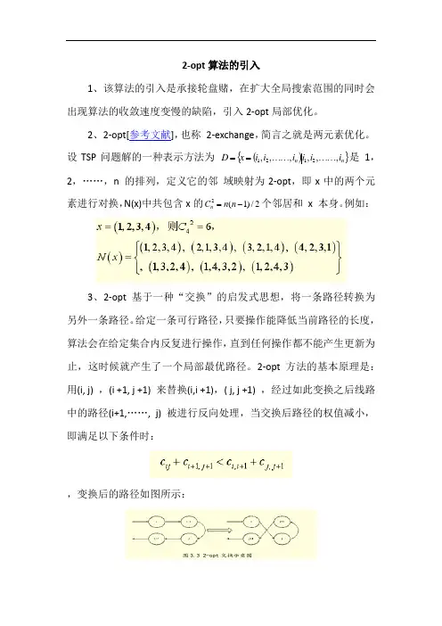
设TSP 问题解的一种表示方法为 (){}n n i i i i i i x D ,,,,,,2121⋯⋯⋯⋯==是 1,
2,……,n 的排列,定义它的邻 域映射为2-opt ,即x 中的两个元素进行对换,N(x)中共包含x 的2/)1(2-=n n C n 个邻居和 x 本身。
例如:
3、2-opt 基于一种“交换”的启发式思想,将一条路径转换为另外一条路径。
给定一条可行路径,只要操作能降低当前路径的长度,算法会在给定集合内反复进行操作,直到任何操作都不能产生更新为止,这时候就产生了一个局部最优路径。
2-opt 方法的基本原理是:用(i, j) ,(i +1, j +1) 来替换(i,i +1),( j, j +1) ,经过如此变换之后线路中的路径(i+1,……, j) 被进行反向处理,当交换后路径的权值减小,即满足以下条件时:
,变换后的路径如图所示:
蚁群算法每次迭代后,在对每个蚂蚁构建的路径使用2-opt方法的过程中,大部分蚂蚁搜索的结果对当前最优解并没有贡献,而当前最优的结果往往来自当前迭代中更短的那些路径,而对最优解没有贡献的路径使用2-opt方法消耗大量的运行时间。
当问题规模和蚂蚁的数量较大,使用2-opt方法会消耗更多的时间。
针对这个问题,在本章改进蚁群算法中,算法在每次迭代后,仅对部分更优的路径使使用2-opt方法,既节省了计算时间,又提高搜索效率。

求解tsp问题的一种改进蚁群算法求解旅行商问题(TSP)一直是计算机科学领域以及应用数学研究中的热门话题,解决TSP问题的方法一直是学术界关注的重点。
本文提出了一种改进的蚁群算法(ICA),该算法利用蒙特卡洛搜索技术,模拟蚁群行为,以获得最优解决方案。
该算法采用带有多种参数控制模型,有助于提高求解TSP问题的效率,从而更好地满足客户需求。
蚁群算法蚁群算法(Ant Colony Algorithm,简称ACA)是一种仿生算法,它模拟了真实蚂蚁的行为,尝试解决TSP问题。
该算法结合了模拟退火法(SA)和遗传算法(GA)的优点,以模拟真实蚂蚁的觅食行为,以寻找最优解决方案。
它利用一组自组织的蚂蚁搜索和定期更新信息素信息,以建立一个索引,使其在搜索空间中更快地找到可行解。
在本文中,我们提出了改进的蚁群算法(ICA),它具有更高的执行效率,能够更好地求解TSP问题。
改进蚁群算法改进的蚁群算法(ICA)是基于原始蚁群算法(ACA)的新框架,它利用蒙特卡洛搜索技术,以模拟蚁群的行为,以寻找最优的解决方案。
该算法使用人工选择算法以动态选取最优路径序列,能够有效地减少求解时间。
此外,ICA利用“参数控制”技术可以调控迭代次数,以获得最优路径序列。
改进的蚁群算法的优势改进的蚁群算法(ICA)有着许多优点,其中最为明显的有:(1)改进的ICA算法在求解TSP问题时,具有更高的执行效率,使得结果更为精确;(2)ICA利用蒙特卡洛搜索技术,通过人工选择算法,以动态选取最优路径序列,有效减少了求解TSP问题的时间;(3)ICA 还采用了“参数控制”,可以有效控制算法的迭代次数,以获得最优路径序列。
实验结果为了检验改进的蚁群算法(ICA)的有效性,我们在不同的计算机环境上进行了实验,并比较了ICA与传统的蚁群算法(ACA)以及其他最新算法(如遗传算法)的性能。
结果表明,ICA要优于传统的蚁群算法。
结论本文提出了一种改进的蚁群算法(ICA),它具有更高的执行效率,能够更好地求解TSP问题。
遗传算法解决tsp问题算法流程下载温馨提示:该文档是我店铺精心编制而成,希望大家下载以后,能够帮助大家解决实际的问题。
文档下载后可定制随意修改,请根据实际需要进行相应的调整和使用,谢谢!并且,本店铺为大家提供各种各样类型的实用资料,如教育随笔、日记赏析、句子摘抄、古诗大全、经典美文、话题作文、工作总结、词语解析、文案摘录、其他资料等等,如想了解不同资料格式和写法,敬请关注!Download tips: This document is carefully compiled by theeditor. I hope that after you download them,they can help yousolve practical problems. The document can be customized andmodified after downloading,please adjust and use it according toactual needs, thank you!In addition, our shop provides you with various types ofpractical materials,such as educational essays, diaryappreciation,sentence excerpts,ancient poems,classic articles,topic composition,work summary,word parsing,copy excerpts,other materials and so on,want to know different data formats andwriting methods,please pay attention!遗传算法解决 TSP 问题的算法流程。
1. 初始化群体。
110 •电子技术与软件工程 Electronic Technology & Software Engineering计算机技术应用• the Application of Computer Technology提供基础信息库的查询功能,在手机建立信息查询专栏,与应用系统进行数据交换以实现查询结果列表。
3.4 日常考勤利用手机的GPS 功能,实现日常考勤签到及工作情况监督,工作人员可以利用手机填写签到表。
利用社区已通的GPS 功能,实现上下班签到、网格巡查监管、未开机监管等工作考勤,并形成统计报表,以便于工作考核。
实现在大屏幕上显示所有网格管理员处在地图上的位置,并用颜色标识。
3.5 信息推送系统自动将部分信息主动推送给相关网格管理员的手机APP 中,例如核查任务,事件催办等,根据对应事件的进度在网格内进行信息提醒。
3.6 事件填报填写事件登记台账表,上传至应用系统中。
3.7 数据交换与应用系统之间实现信息交换,获取网格内相关人员、法人、房屋、城市部件配置等方面信息,制定交换的标准格式,交换方式等内容。
利用JSON 格式,实现数据交换的标准管理,JSON 格式可为Javascript 、Java 、Andriord 、IOS 等环境支持。
3.8 网格地图浏览网格地图基本操作,使用ARCGIS 地图,提供符合大多数用户使用习惯的电子地图的放大、缩小、移动、搜索等功能。
3.9 电子巡更巡查记录包括联动部门巡查人员的巡查轨迹的查看和社区网格巡查人员的巡查轨迹的查看。
街道、村/社区工作人员安装APP 后,PC 系统会在工作时间自动记录工作人员的巡查路径、时间并与GPS 数据进行匹配,以确定是否按规定进行巡查。
3.10 电子走访网格工作人员用APP 扫描居民住宅楼道或数字电视平台上的二维码后,进入电子巡更界面,选择“走访类型”后,系统数据库自动记录这次走访的时间、被走访居民家庭信息、工作人员信息等内容,被走访居民居住地GIS地理信息。
tsp问题的memetic求解算法
TSP问题(Traveling Salesman Problem)是一种著名的组合优化问题,通常被认为是NP难问题。
它的目标是给定一组城市和它们之间的距离,寻找一条遍历所有城市仅一次的最短路径。
由于该问题难度很大,所
以需要一种高效的求解算法。
Memetic算法是一种基于遗传算法和局部搜
索相结合的优化算法,已被证明在TSP问题上有很好的效果。
Memetic算法的基本步骤如下:
1.初始化种群:随机生成一些初始解作为种群,并为每个解分配一个
初始适应度值。
2.进化操作:使用遗传算法进行进化操作,即选择、交叉和变异。
选
择操作选出优秀的个体进行遗传,交叉操作将两个个体的染色体进行交叉
以产生新的个体,变异操作对染色体进行随机变化以引入新的搜索方向。
3. 局部搜索:对个体进行局部搜索以优化解的质量。
这里使用2-
opt算法作为局部搜索算法,它可以对一条路径进行优化,去除其中的交
叉边,以达到更优的路径。
4.更新适应度:根据优化后的个体重新计算适应度值,以更新种群。
5.结束条件:达到预设的结束条件,例如达到了规定的迭代次数或者
找到了满足要求的解等。
传统的Memetic算法存在随机性比较大的缺陷,容易陷入局部最优解。
因此,一些优化方法被提出来,例如:改进交叉算子、多种子种群、领域
小环境等等,以提高该算法的效率和稳定性。
总之,Memetic算法是一种优秀的求解TSP问题的算法,尤其是结合了局部搜索和遗传算法的优点,可以在搜索空间较大的情况下获得更好的搜索结果。
TSP的几种求解方法及其优缺点旅行商问题(TSP)是一个组合优化问题,目的是找到一条最短的路径,使得旅行商能够访问一系列城市并返回起始点。
TSP由于其复杂性而被广泛研究,已经发展出了许多求解方法。
本文将讨论几种主要的TSP求解方法,包括贪婪算法、局部算法、遗传算法和蚁群算法,并分析它们的优缺点。
1.贪婪算法贪婪算法是一种基于贪心策略的求解方法。
它从一个起始城市开始,每次选择距离当前城市最近的未被访问过的城市作为下一步的目标城市,直到所有的城市都被访问过。
贪婪算法的优点是简单易于理解和实现,并且在处理小规模问题时效果显著。
然而,贪婪算法没有考虑全局最优解,很容易陷入局部最优解,不能保证找到最优解。
2.局部算法局部算法是一类启发式算法,它通过不断优化当前解来逐步接近最优解。
其中最典型的是2-opt算法,它通过交换路径中的两个顶点位置来改进解的质量。
局部算法的优点是可以找到局部最优解,且计算时间较短。
然而,局部算法容易陷入局部最优解,而且计算开销随问题规模增加而增加,且不能保证找到全局最优解。
3.遗传算法遗传算法是一种模拟生物进化的随机算法。
它通过模拟遗传、交叉和变异等基因操作来生成和改进解。
遗传算法的优点是可以处理大规模问题,且不容易陷入局部最优解。
同时,遗传算法能够在空间中探索多个解,提高解的多样性。
然而,遗传算法的计算开销相对较高,需要大量的迭代和种群更新。
此外,遗传算法的性能与参数设置相关,需要进行调整。
4.蚁群算法蚁群算法是一种模拟蚂蚁觅食行为的算法。
它通过模拟蚂蚁在路径上释放信息素的过程,来引导蚂蚁选择路径。
蚁群算法的优点是能够找到较好的解并具有一定的自适应性。
它适用于处理大规模问题,且能够处理问题中的不确定性。
然而,蚁群算法的计算开销较高,并且参数设置对结果影响较大。
综上所述,TSP的求解方法包括贪婪算法、局部算法、遗传算法和蚁群算法等。
每种方法都有自己的优点和缺点。
选择适合问题规模、问题特征和求解时间的方法是关键。
TSP资料处理结果的可靠性评估方法TSP(Traveling Salesman Problem,旅行推销员问题)是组合优化问题中的一个经典问题,该问题要求在给定一系列城市和两两之间的距离矩阵之后,寻找一条最短的路径,使得旅行推销员能够访问每个城市一次并回到起始城市。
在解决TSP问题时,数据处理结果的可靠性评估是非常重要的。
下面将介绍几种常见的TSP数据处理结果的可靠性评估方法:1.基于启发式算法的评估方法:TSP问题的规模非常庞大,准确求解通常不可行。
因此,常常采用启发式算法求解,并通过比较不同算法得到的结果来进行评估。
常用的启发式算法包括贪婪算法、禁忌和遗传算法等。
可以通过运行不同的启发式算法多次,比较它们的结果来评估数据处理结果的可靠性。
2.比较与已知最优解的偏差:对于一些特定规模较小的问题,可以通过计算与已知最优解的偏差来评估数据处理结果的可靠性。
已知最优解可以通过暴力、精确求解或通过计算最优路径的上界等方法获得。
3.重复计算结果的评估方法:对于TSP问题,由于问题的复杂性,算法可能陷入局部最优。
因此,处理结果的可靠性评估需要对算法进行多次重复计算。
通过多次计算结果的均值、方差等统计指标来评估数据处理结果的可靠性。
4.交叉验证的评估方法:交叉验证是一种常用的机器学习中的评估方法,可以用于评估TSP数据处理结果的可靠性。
将数据分成训练集和测试集,训练集用于选择算法的参数和训练模型,测试集用于评估模型的性能。
通过多次随机划分训练集和测试集,计算评估指标的均值和方差,可以评估数据处理结果的可靠性。
5.对假设进行检验的评估方法:对于TSP问题,可以对一些关键假设进行检验来评估数据处理结果的可靠性。
例如,可以检验最优路径中每个城市只出现一次的假设,如果存在重复访问城市的情况,则说明结果不可靠。
综上所述,TSP数据处理结果的可靠性评估方法包括基于启发式算法的评估方法、比较与已知最优解的偏差、重复计算结果的评估方法、交叉验证的评估方法和对假设进行检验的评估方法等。
Comparison of TSP AlgorithmsProject forModels in Facilities Planning andMaterials HandlingDecember 1998Participants:Byung-In KimJae-Ik ShimMin ZhangExecutive SummaryOur purpose in this term project is to implement heuristic algorithms and compare and evaluate their respective computational efficiency. Included in this model are greedy, 2-opt, greedy 2-opt, 3-opt, greedy 3-opt, genetic algorithm, simulated annealing, and neural network approach and their improvement versions. The problem size can be adjusted from 2-node up to 10,000-node. Therefore, these algorithms can be evaluated in a wide spectrum of situations.We implemented above heuristic algorithms. The conclusion that is derived from this project is for small-size TSP (n≤50), greedy 2-opt algorithm performs pretty well, i.e high optimality vs. little computational time. The neural network(Self Organizing feature Maps) algorithm shows the best efficiency for all city sizes.Furthermore the algorithms were improved by using non crossing methods. This improved methods always result in better solutionsTable of Content1. Introduction2. Description of AlgorithmsA. GreedyB. 2-OptC. Greedy 2-OptD. 3-OptE. Greedy 3-OptF. GeneticG. Simulated AnnealingH. Neural Network3. Improvement of Algorithms4. Simulation Results and Analysis5. Conclusion6. ReferenceAppendix (Programming Code)1. IntroductionThe Travelling Salesman Problem (TSP) is a deceptively simple combinatorial problem. It can be stated very simply: A salesman spends his time visiting N cities (or nodes) cyclically. In one tour he visits each city just once, and finishes up where he started. In what order should he visit them to minimize the distance traveled? TSP is applied in many different places such as warehousing, material handling and facility planning.Although optimal algorithms exist for solving the TSP, like the IP formulation, industrial engineers have realized that it is computationally infeasible to obtain the optimal solution to TSP. And it has been proved that for large-size TSP, it is almost impossible to generate an optimal solution within a reasonable amount of time. Heuristics, instead of optimal algorithms, are extensively used to solved such problems. People conceived many heuristic algorithms to get near-optimal solutions. Among them, there are greedy, 2-opt, 3-opt, simulated annealing, genetic algorithms, neural network approach, etc. But their efficiencies vary from case to case, from size to size.The algorithms can be implemented by using Visual C++. From these program the results are attained and the results of each algorithms can be compared. These algorithms can be improved by using the non-crossing method which is explained in “Improvement Algorithm”. The comparison of the results shows the optimality of each algorithm varies with the problem size.2. Description of AlgorithmsThe heuristic algorithms for TSP can be classified as1. Construction Algorithms;2. Improvement Algorithms; and3. Hybrid Algorithms.Construction algorithms are those in which the tour is constructed by including points in the tours, usually one at a time, until a complete tour is developed. In improvement algorithms, a given initial solution is improved, if possible, by transposing two or more points in the initial tour. With regard to improvement algorithms, two strategies are possible. We may either consider all possible exchanges and choose the one that results in the greatest savings and continue this process until no further reduction is possible; or as soon as a savings is available, we may make the exchange and examine other possible exchanges and keep the process until we cannot improve the solutions any further. In our project, the former are 2-opt and 3-opt algorithms; and the latter are greedy 2-opt and greedy 3-opt algorithms. Hybrid algorithms use a construction algorithms to obtain an initial solution and then improve it using an improvement algorithm. In our project, simulated annealing and neural network fall into this category.A. Greedy AlgorithmGreedy algorithm is the simplest improvement algorithm. It starts with the departure Node 1. Then the algorithm calculates all the distances to other n-1 nodes. Go to the next closest node. Take the current node as the departing node, and select the next nearest node from the remaining n-2 nodes. The process continues until all the nodes are visited once and only once then back to Node 1. When the algorithm is terminated, the sequence is returned as the best tour; and its associated OFV is the final solution. The advantage of this algorithm is its simplicity to understand and implement. Sometime, it may lead to a very good solution when the problem size is small. Also, because this algorithm does not entail any exchange of nodes, it saves considerably much computational time.For the C++ code for greedy algorithm, please refer to the Appendix.B. 2-Opt AlgorithmFor n nodes in the TSP problem, the 2-Opt algorithm consists of three steps:Step 1Let S be the initial solution provided by the user and z its objective function value (In our model, we use greedy algorithm to setup the initial solution and objective function value.). Set S*=s, z*=z, i=1 and j=i+1=2.Step 2Consider the exchange results in a solution S’ that has OFV z’<z*, set z*=z’ and S*=S’. If j<n repeat step 2; otherwise set i=i+1 and j=i+1. If i<n, repeat step 2; otherwise go to step 3.Step 3If S≠S*, set S=S*, z=z*, i=1, j=i+1=2 and go to step 2. Otherwise, output S* as the best solution and terminate the process.Observe that the 2-opt algorithm considers only pairwise exchange. Initially, the algorithm considers transposition of Nodes 1 and 2. If the resulting solution’s OFV is smaller than that of the initial solution, it is stored as a candidate for future consideration. If not, it is discarded and the algorithm considers transposing of Nodes 1 and 3. If this exchange generates a better solution, it is stored as a candidate for future consideration; if not, it is discarded. Thus, whenever a better solution is found, the algorithm discards the previous best solution. This procedure continues until all the pairwise exchanges are considered. Because each node can be exchanged with n-1 other nodes and there are n nodes in total, there are n(n-1)/2 different exchanges. These n(n-1)/2 exchanges are considered in step 2. The solution retained at the end of step 2 is the one that provides the most improvement in the OFV. Starting with this as the new solution, the algorithm repeats step 2 to find another better solution. At some stage, no improvement in the current best solution is possible, and then the algorithm terminates. The remaining solution is returned to the user as the best one.For the C++ code for 2-opt algorithm, please refer to the Appendix.C. Greedy 2-Opt AlgorithmThe greedy 2-Opt algorithm is a variant of 2-opt algorithm. It also consists of three steps:Step 1Let S be the initial solution provided by the user and z its objective function value (In our model, we use greedy algorithm to setup the initial solution and objective function value.). Set S*=s, z*=z, i=1 and j=i+1=2.Step 2Transpose Node i and Node j, i<j. Compare the resulting OFV z with z*. If z ≥ z* and j<n, set j=j+1 and repeat step 2; Otherwise go to step 3.Step 3If z<z*, set S*=S, z*=z, i=1, j=i+1=2 and go to step 2. If z ≥ z* and j=n, set i=i+1, j=j+1 and repeat step 2. Otherwise, output S* as the best solution and terminate the process.Like the 2-Opt algorithm, greedy 2-opt algorithm also considers pairwise exchanges. Initially, it considers transposing Nodes 1 and 2. If the resulting OFV is less than the previous one, two nodes are immediately transposed. If not, the algorithm will go on to Node 3 and evaluate the exchange, and so on until find the improvement. If Nodes 1 and 2 are transposed, the algorithm will take it as an initial solution and repeat the algorithm until it is impossible to improve the solution any further. Greedy 2-opt algorithm makes the exchange permanent whenever an improvement is found and thus consumes less computational time than 2-Opt algorithm. On the other hand, greedy 2-opt produces slightly worse solutions than 2-Opt algorithm.For the C++ code for greedy 2-opt algorithm, please refer to the Appendix.D. 3-Opt AlgorithmThe 3-Opt algorithm is similar to the 2-opt algorithm except that it considers transposing two nodes at a time. There are two possible ways of transposition.: i->j->k->iand j->k->i->j. Let’s just consider the first transposition. The steps involved are Step 1.Let S be the initial solution and z its OFV. Set S*=S,z*=z,i=1,j=i+1 and k=j+1.Step 2. Consider transposing Nodes i, j, k in “i->j->k->i” fashion. If the resulting solution S’ has a smaller z’<z*, set z*=z’ and S*=S’. If k<n, set k=k+1. Otherwise, set j=j+1. If j<n-1, set k=j+1. Otherwise, set i=i+1, j=j+1 and k=j+1. If i<n-2, repeat step 2. Otherwise go to step 3.Step 3If S≠S*, set S=S*, z=z*, i=1, j=i+1,k=j+1 and go to step 2. Otherwise, output S* as the best solution and terminate the process.For the C++ code for 3-Opt algorithm, please refer to the Appendix.E.Greedy 3-Opt AlgorithmLike the greedy 2-opt algorithm, greedy 3-opt algorithm also makes the 3-node exchange permanent whenever its resulting OFV is better than the currentOFV and repeats the algorithm with the new transposition as the initial solution. Let’s just consider the “i->j->k->i” transposition again. The steps involved are: Step 1Let S be the initial solution provided by the user and z its objective function value (In our model, we use greedy algorithm to setup the initial solution and objective function value.). Set S*=S,z*=z,i=1,j=i+1 and k=j+1.Step 2. Consider transposing Nodes i, j, k in “i->j->k->i” fashion. If the resulting solution S’ has a smaller z’<z*, set z*=z’ and S*=S’. If k<n, set k=k+1. Otherwise, set j=j+1. If j<n-1, set k=j+1. Otherwise, set i=i+1, j=j+1 and k=j+1. If i<n-2, repeat step 2. Otherwise go to step 3.Step 3If z<z*, set S*=S, z*=z, i=1, j=i+1=2, k=j+1 and go to step 2. If z ≥ z* and k=n, set i=i+1, j=j+1, and repeat step 2. . If z ≥ z* and j=n-1, set i=i+1, and repeat step 2. Otherwise, output S* as the best solution and terminate the processThe advantage of greedy 3-Opt algorithm over 3-Opt algorithm is once again less computational time due to its less thorough search in the network.For the C++ code for greedy 3-Opt algorithm, please refer to the Appendix.F. Genetic AlgorithmAs the name implies, this algorithm gets its idea from genetics. The algorithm works this way.Step 0Obtain the maximum number of individuals in the population P and the maximum number of generations G from the user, generate P solutions for the first generation’s population randomly, and represent each solution as a string. Set generation counter N gen=1.Step 1Determine the fitness of each solution in the current generation’s population and record the string that has the best fitness.Step 2 Generate solutions for the next generation’s population as follows:1. Retain 0.1P of the solutions with the best fitness in the previouspopulation.2. Generate 0.89P solutions via mating, and3. Select 0.01P solutions from the previous population randomly andmutate them.Step 3 Update N gen=N gen+1. If N gen≤G, go to Step 1. Otherwise stop.In our project, we used the two-point crossover method, given two parent chromosomes {x1,x2,….x n} and {y1,y2,…,y n}, two integers r and s are randomly selected, such that 1 ≤ r ≤ s ≤ n. And the genes in positions r to s of one parent are swapped with those of the other to get two offsprings as follows.{x1, x2,…, x r-1, y r, y r+1,…, y s, x s+1, x s+2,…, x n}{y1, y2,…, y r-1, x r, x r+1,…, x s, y s+1, y s+2,…, y n}Either both or the better of the two offspring is then included in the new population. This mutation procedure is repeated until the required number of offspring is generated. To avoid generating infeasible solutions, we also used thepartially matched crossover method. Set t=r, and swaps genes x t and y t if x t≠y t in the first parent x={x1, x2,…, x r-1, x r, x r+1,…, x s, x s+1, x s+2,…, x n}. This swapping is done for t=r through s, one by one, and then we have a feasible offspring. The same is done for y={y1, y2,…, y r-1, y r, y r+1,…, y s, y s+1,y s+2,…, y n}. Because the partially matched crossover method always swaps genes within a parent, feasible offspring are obtained.Therefore, our model uses mutation to generate a population by swapping any two randomly selected genes.For the C++ code for genetic algorithm, please refer to the Appendix.H. Simulated AnnealingThe basic idea of simulated annealing(SA) is from the statistical mechanics and is motivated by an analogy of behavior of physical systems in the presents of a heat bath. This algorithm obtains better final solutions by gradually going from one solution to the next. The main difference of SA from the 2-opt or 3-opt algorithm is that the local optimization algorithm is often restrict their search for the optimal solution in a downhill direction which mean that the initial solution is changed only if it results in a decrease in the OFV. The temperature refers to the state through which the simulated annealing algorithm passes in its search for a better solution. Starting with an initial temperature, we move to the next temperature only when we have reached a frozen state. When a frozen state is reached, the temperature is reduced by a cooling factor r, and the procedure is repeated until a certain predetermined number of temperature steps have been performed.Step 0Set S = initial feasible solutionz = corresponding OFVT = initial temperature = 1; r = cooling factor = 0.9ITEMP = number of times the temperature T is decreased = 0NLIMIT = maximum number of new solutions to be accepted ateach temperature = 10nNOVER = maximum number of solutions evaluated at eachtemperature = 100nStep 1Repeat step 2 NOVER times or until the number of successful new solutions is equal to NLIMITStep2Pick a pair of machines randomly and exchange their positions. If the exchange of the position of the two machines results in the overlapping of some other pairs of cities, appropriately modify the coordinates of the center of the concerned machines to ensure no overlapping. If the resulting solution S* has OFV <= z, set S* = S and z = corresponding OFV. Otherwise, compute delta = difference between z and the OFV of the solution S*. and set S*=S with a probability e-delta/T .Step 3 Set T = rT and ITEMP = ITEMP + 1. If ITEMP <= 100, go to step 1;otherwise stop.For the C++ code for simulated annealing algorithm, please refer to the Appendix.G. Neural Network(Self Organizing Feature Maps)First, randomly pick up any city in the network as the initial loop. The number of nodes N on the loop grows subsequently according to a node creation process. (see below). At each processing step, a city i is surveyed. One complete iteration takes M (number of total cities to be visited) sequential steps, for i=1 to i=M, thus picking every city once in a preset order. A gain parameter is used which decreases between two complete iterations. Several iterations are needed to go from the high gain value to the low one giving the final result.Surveying the city i comprises the following steps:Step 1. Find the node j c which is closed to city i.Step 2.Move node j c and its neighbors on the ring towards city i. The distance each node will move is determined by a function f(G,n) where G is the gain parameter (its initial is set 10 in our model), and n is the distance measured along the loop between nodes j and j c.n=inf (j- j c (mod N), j c -j(mod N))Every node j is moved from current position to a new one.The function f is defined to bef(G,n)=sqrt(1/2)*exp(-n2/G2)This means:- when G →∞, all nodes move towards city I with the same strength sqrt(1/2).- when G → 0, only node jc moves towards city i.Decreasing the gain at the end of a complete survey is done by G←(1-α)G. α is the only parameter that has to be adjusted. It is directly related to the number of complete surveys needed to attain the result, and hence its quality.The gain is decreased from a high initial G i which ensures large moves for all nodes at each iteration step to a sufficiently low G f for which the network is stabilized. The total number of iterations can be computed from these two fixed values depending only on M.A node is duplicated, if it is chosen as the winner for two different cities in the same complete survey. The newly created node is inserted into the ring as a neighbor of the winner, and with the same coordinates in the plane. Both the winner and the created node are inhibited. If chose by a city, an inhibited node will induce no movement at all in the network for this city presentation. It is re-enabled on the next presentation. This guarantees that the “twin nodes” will be separated by the moves of their neighbors, before being “caught” by cities. The maximum number of nodes created on the loop experimentally appears to be less than 2M.A node is deleted, if it has not been chosen as the winner by any city during three complete surveys. This creation-deletion mechanism has proved important to the attainment of near-optimum solutions.For the C++ code for neural network approach, please refer to the Appendix.3. Improvement of AlgorithmsIn the initial implementation of these 8 algorithms, it is found that these algorithms do not eliminate the crossing of routes. Of course, these crossings of routes lengthen the total distance of travel in TSP. We improved these algorithms by getting rid of these crossings.The process is as follows.First, obtain the solution with any of the preceding algorithms. Second, pick up the segment between Node 1 and Node 2, check any other segment against the 1-2 segment to see if these 2 segments intersect each other. If not, pick up the segment 2-3, and check consequent segment against segment 2-3. If the intersection is found for any two distinct segments, re-route the loop. And the process is continued sequentially throughout the network.The mathematical implementation of both checking and re-routing is as follows: The current 2 segments are i→i+1, j→j+1 (1 ≤ i < i+1 < j< j+1 ≤ n). The line of i→i+1 segment can be expressed as x=x i+(x i-1 - x i)*t, y= y i +(y i+1 - y i)*t, and the line of j→j+1 segment can be expressed as x=x j+(x j-1 - x j)*s, y= y j +(y j+1-y j)*s. Given these parametric expressions and the coordinates of these 4 nodes, the coordinates and associated s, and t can be calculated for the intersection of these lines. If both s and t are0 ≤ t ≤ 1 and 0 ≤ s ≤ 1, it is determined that these two segments are intersected. Otherwise not. When they are intersected, transpose node i+1 and node j. There would be neither intersection on these 2 segments nor break of the loop.Since there are N+1 routes for N cities, N(N+1)/2 crossing-checks are necessary. Our model finds these non-crossing methods substantially improved upon these algorithms for large-size problem.( Original Result )( Improved Result )4. Implementation & AnalysisWe implemented above algorithms by using Microsoft Visual C++ 5.0 ( with MFC library ). The main menu and windows are followed. <TSP menu> is menu for solving TSP by using several algorithms and <TSP Result View> is menu for viewing the results.1) make DataOur program can get the city number from user and make cities’ locations by using random generation function. We fixed the maximum X and Y values to 500.2) Greedy algorithm and Improved Greedy algorithmLength : 4478.38Length : 4335.93Time : 0 sec3) Greedy 2-OPT and Improved Greedy 2-OPTLength : 4477.87Length : 4128.87 Time : 0 sec4) 2-OPT and Improved 2-OPTLength : 4320.34Length : 4122.58 Time : 0 sec5) Greedy 3-OPT and Improved Greedy 3-OPTLength : 4356.92Length : 4124.95 Time : 11 sec6) 3-OPT and Improved 3-OPTLength : 4356.92Length : 4124.95 Time : 30 sec7) Simulated Annealing and Improved Simulated AnnealingLength : 4320.42Length : 4122.65Time : 6 sec8) Genetic Algorithm and Improved Genetic AlgorithmThe user can give Population size and generation size like following dialogFollowing results used population size 100 and generation size 100Length : 4302.99Length : 4200.69Time : 8 sec9) Neural Network(Self Organized Feature Map) and Improved Neural NetworkLength : 4035.32Length : 43995.19Time : 12 sec500 cities caseLength : 8778.29Time : 346 secLength : 8773.8510 ) AnalysisWe did a performance comparison of 8 algorithms and improved versions. For the simulation city size of 30, 100 and 500 were used. The below tables and graphs illustrate the result of simulation. The neural network algorithm came up with the shortest distance for all the number of cities. The improved version of the algorithms always resulted in better solution compared to the original solution. For the time of simulation, 3-Opt and Greedy 3-Opt had the longest time to find the solution. That is why for 500 cities, these algorithms did not give the solution. As the number of the cites increased the simulation time also increased for some of the algorithms. Excluding the 3-Opt and Greedy 3-Opt, the neural network took the longest time to simulate for 500 cites which was 346 seconds.< Length Comparison >Algorithm \ City Size30100500Greedy2330447810402Improved Greedy2187433510279Greedy 2-OPT2095437710127Improved Greedy 2-OPT2095412895002-OPT2095432010083Improved 2-OPT209541229459Greedy 3-OPT22404356Improved Greedy 3-OPT216841243-OPT21784356Improved 3-OPT21554124Simulated Annealing2177432010279Improved Simulated213141229606AnnealingGenetic Algorithm229543029906Improved Genetic220142009364AlgorithmNeural Network208640358778Improved Neural Network208639958773< Time Comparison >Algorithm \ City Size30100500Greedy001Greedy 2-OPT0022-OPT0014Greedy 3-OPT0113-OPT030Simulated Annealing2627Genetic Algorithm6834Neural Network112346< Length Comparison >< Time Comparison >5. ConclusionWe implemented the above-mentioned heuristic algorithms. It is shown that the algorithms were improved by using non crossing methods. This improved methods always result in better solutions. The conclusion that is derived from this project is for small-size TSP (n≤50), greedy 2-opt algorithm performs pretty well, i.e high optimality vs. little computational time. The neural network(Self Organizing feature Maps) algorithm demonstrates the best efficiency for all city sizes. Through the simulation, the improved neural network algorithm gives us the shortest distance for 30 cities, 100 cities and 500cities. The number of the cities doesn’t affect the optimality of algorithms. Therefore no matter how many cities are involved in the Travelling salesman problem, the Neural network algorithm will give the best solution of all these 16 algorithms that were mentioned in this report. The simulation of 3-Opt algorithm take a very long time for a large number of cities such as 500. It is not efficient to use 3-Opt algorithm for problem with more than 100 cites.For small-size TSP (n≤50), improved greedy 2-opt algorithm is recommended. For medium-size TSP (50≤n≤100), improved 2-opt algorithm and neural network are recommended for their optimality and efficiency. For large-size problem (100≤n≤500), the improved genetic algorithm is recommended. For any problem-size, if the computational time is not a constraint, the improved neural network is always recommended.6. ReferencesAngeniol, B., Vaubois, G de L C. and Texier JYL.(1988) Self-Organizing Feature Maps and the Traveling Salesman Problem, Neural Networks, Vol 1, pp 289-293.Heragu, Sunderesh (1997) Facilities Design, PWS Publishing Company, Boston, MA.。