Optimization Methods

优化方法英语作文Optimization Methods。

Optimization methods refer to a set of techniques used to find the best possible solution to a problem. These methods are widely used in various fields, such as engineering, economics, finance, and computer science. In this article, we will discuss some of the most commonly used optimization methods and their applications.1. Linear Programming。

Linear programming is a mathematical technique used to optimize a linear objective function, subject to linear constraints. It is widely used in business and economics to solve problems related to resource allocation, production planning, and transportation. Linear programming is also used in engineering to optimize the design of structures and systems.2. Nonlinear Programming。

Nonlinear programming is a mathematical technique used to optimize a nonlinear objective function, subject to nonlinear constraints. It is used in a wide range of applications, such as engineering design, chemical process optimization, and financial portfolio optimization. Nonlinear programming is a more complex and challenging optimization method than linear programming, but it allows for more accurate modeling of real-world problems.3. Genetic Algorithms。

连续体结构的拓扑优化设计一、本文概述Overview of this article随着科技的不断进步和工程需求的日益增长，连续体结构的拓扑优化设计已成为现代工程领域的研究热点。

拓扑优化旨在通过改变结构的内部布局和连接方式，实现结构性能的最优化，从而提高工程结构的承载能力和效率。

本文将对连续体结构的拓扑优化设计进行深入研究，探讨其基本原理、方法、应用以及未来的发展趋势。

With the continuous progress of technology and the increasing demand for engineering, the topology optimization design of continuum structures has become a research hotspot in the field of modern engineering. Topology optimization aims to optimize the structural performance by changing the internal layout and connection methods of the structure, thereby improving the load-bearing capacity and efficiency of engineering structures. This article will conduct in-depth research on the topology optimization design of continuum structures, exploring their basic principles, methods,applications, and future development trends.本文将介绍连续体结构拓扑优化的基本概念和原理，包括拓扑优化的定义、目标函数和约束条件等。

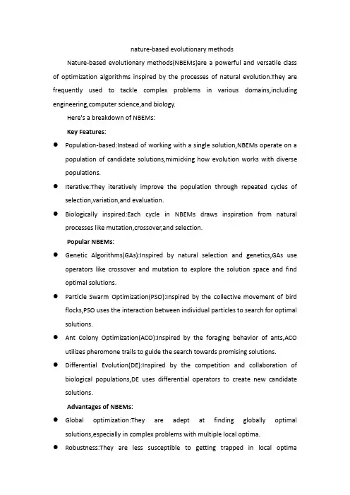
nature-based evolutionary methodsNature-based evolutionary methods(NBEMs)are a powerful and versatile class of optimization algorithms inspired by the processes of natural evolution.They are frequently used to tackle complex problems in various domains,including engineering,computer science,and biology.Here's a breakdown of NBEMs:Key Features:●Population-based:Instead of working with a single solution,NBEMs operate on apopulation of candidate solutions,mimicking how evolution works with diverse populations.●Iterative:They iteratively improve the population through repeated cycles ofselection,variation,and evaluation.●Biologically inspired:Each cycle in NBEMs draws inspiration from naturalprocesses like mutation,crossover,and selection.Popular NBEMs:●Genetic Algorithms(GAs):Inspired by natural selection and genetics,GAs useoperators like crossover and mutation to explore the solution space and find optimal solutions.●Particle Swarm Optimization(PSO):Inspired by the collective movement of birdflocks,PSO uses the interaction between individual particles to search for optimal solutions.●Ant Colony Optimization(ACO):Inspired by the foraging behavior of ants,ACOutilizes pheromone trails to guide the search towards promising solutions.●Differential Evolution(DE):Inspired by the competition and collaboration ofbiological populations,DE uses differential operators to create new candidate solutions.Advantages of NBEMs:●Global optimization:They are adept at finding globally optimalsolutions,especially in complex problems with multiple local optima.●Robustness:They are less susceptible to getting trapped in local optimacompared to traditional optimization methods.●Adaptability:They can be adapted to handle a wide range of optimizationproblems with varying constraints and objectives.Challenges of NBEMs:●Computational cost:They can be computationally expensive,especially for largepopulations and complex problems.●Parameter tuning:Choosing appropriate parameter settings can significantlyimpact the performance of NBEMs.●Lack of theoretical guarantees:Unlike some traditional optimizationmethods,NBEMs often lack strong theoretical guarantees of convergence.Applications of NBEMs:●Engineering design:NBEMs are used to optimize the design ofstructures,machines,and materials.●Scheduling and resource allocation:They help optimize schedules for tasks andallocate resources efficiently.●Machine learning:NBEMs can be used to optimize hyperparameters in machinelearning models.●Data mining and analysis:They can be used to discover patterns and trends inlarge datasets.Conclusion:NBEMs are a valuable tool for tackling complex optimization problems in diverse domains.Their ability to find globally optimal solutions,adapt to different problems,and handle diverse constraints makes them a powerful and versatile choice.However,it's important to consider their computational cost,parameter tuning requirements,and lack of strong theoretical guarantees when deciding if they are suitable for a specific problem.。

智能优化算法英文投稿选类别
智能优化算法的英文投稿在选择类别时，可以考虑以下几个类别：
1. Artificial Intelligence (人工智能)：这个类别涵盖了所有形式的人工智能技术，包括但不限于机器学习、深度学习、强化学习、神经网络等。

如果你的智能优化算法是基于某种人工智能技术，那么这个类别可能非常适合。

2. Optimization Methods (优化方法)：这个类别主要关注各种优化算法和技术，包括但不限于遗传算法、粒子群优化、模拟退火、蚁群优化等。

如果你的智能优化算法是一种新的优化方法，那么这个类别可能非常适合。

3. Computer Science (计算机科学)：这个类别涵盖了计算机科学的各个方面，包括算法设计、数据结构、计算复杂性等。

如果你的智能优化算法是一种新的计算方法或者对现有的计算方法进行了改进，那么这个类别可能非常适合。

4. Engineering (工程)：这个类别主要关注实际应用和工程问题，包括但不限于机械工程、航空航天工程、土木工程等。

如果你的智能优化算法是用于解决某个工程问题，那么这个类别可能非常适合。

需要注意的是，选择类别时还需要考虑期刊或会议的投稿要求和规范。

有些期刊或会议可能对稿件的格式、内容、长度等方面有特定的要求，因此在选择类别时需要仔细阅读投稿指南并遵循相关规定。

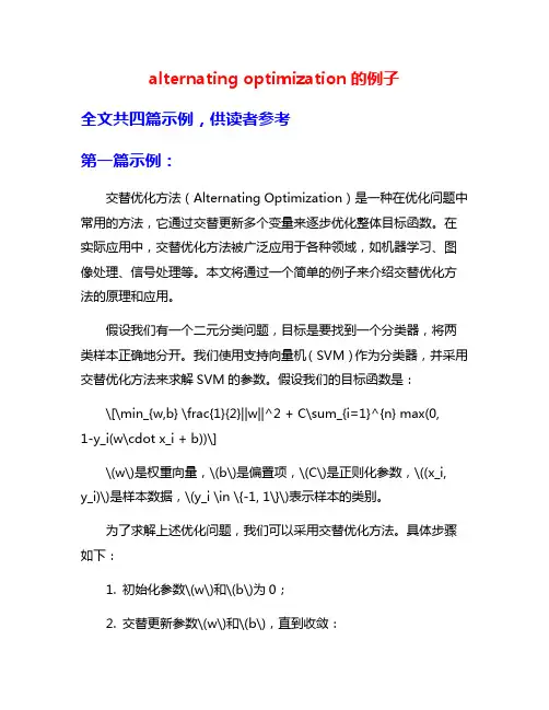
alternating optimization的例子全文共四篇示例，供读者参考第一篇示例：交替优化方法（Alternating Optimization）是一种在优化问题中常用的方法，它通过交替更新多个变量来逐步优化整体目标函数。

在实际应用中，交替优化方法被广泛应用于各种领域，如机器学习、图像处理、信号处理等。

本文将通过一个简单的例子来介绍交替优化方法的原理和应用。

假设我们有一个二元分类问题，目标是要找到一个分类器，将两类样本正确地分开。

我们使用支持向量机（SVM）作为分类器，并采用交替优化方法来求解SVM的参数。

假设我们的目标函数是：\[\min_{w,b} \frac{1}{2}||w||^2 + C\sum_{i=1}^{n} max(0,1-y_i(w\cdot x_i + b))\]\(w\)是权重向量，\(b\)是偏置项，\(C\)是正则化参数，\((x_i,y_i)\)是样本数据，\(y_i \in \{-1, 1\}\)表示样本的类别。

为了求解上述优化问题，我们可以采用交替优化方法。

具体步骤如下：1. 初始化参数\(w\)和\(b\)为0；2. 交替更新参数\(w\)和\(b\)，直到收敛：- 固定\(b\)，更新\(w\)：根据上述目标函数的梯度，我们可以用梯度下降法更新权重向量\(w\)；- 固定\(w\)，更新\(b\)：更新偏置项\(b\)，使得约束条件\(1-y_i(w\cdot x_i + b) \leq 0\)成立；3. 重复步骤2，直到收敛。

通过交替更新\(w\)和\(b\)，我们可以逐步优化SVM的参数，使得分类器能够更好地拟合训练数据，并达到更好的分类性能。

交替优化方法的优点在于它能够在参数空间中高效地搜索最优解，同时能够处理复杂的非凸优化问题。

除了在机器学习中的应用，交替优化方法还被广泛应用于其他领域。

在图像处理中，交替优化方法可以用于图像去噪、图像超分辨率、图像分割等任务中。

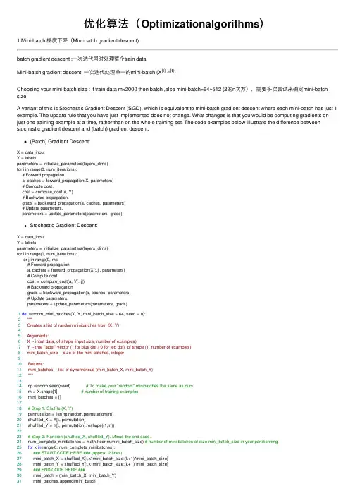
优化算法（Optimizationalgorithms）1.Mini-batch 梯度下降（Mini-batch gradient descent)batch gradient descent :⼀次迭代同时处理整个train dataMini-batch gradient descent: ⼀次迭代处理单⼀的mini-batch (X{t} ,Y{t})Choosing your mini-batch size : if train data m<2000 then batch ,else mini-batch=64~512 (2的n次⽅），需要多次尝试来确定mini-batch sizeA variant of this is Stochastic Gradient Descent (SGD), which is equivalent to mini-batch gradient descent where each mini-batch has just 1 example. The update rule that you have just implemented does not change. What changes is that you would be computing gradients on just one training example at a time, rather than on the whole training set. The code examples below illustrate the difference between stochastic gradient descent and (batch) gradient descent.(Batch) Gradient Descent:X = data_inputY = labelsparameters = initialize_parameters(layers_dims)for i in range(0, num_iterations):# Forward propagationa, caches = forward_propagation(X, parameters)# Compute cost.cost = compute_cost(a, Y)# Backward propagation.grads = backward_propagation(a, caches, parameters)# Update parameters.parameters = update_parameters(parameters, grads)Stochastic Gradient Descent:X = data_inputY = labelsparameters = initialize_parameters(layers_dims)for i in range(0, num_iterations):for j in range(0, m):# Forward propagationa, caches = forward_propagation(X[:,j], parameters)# Compute costcost = compute_cost(a, Y[:,j])# Backward propagationgrads = backward_propagation(a, caches, parameters)# Update parameters.parameters = update_parameters(parameters, grads)1def random_mini_batches(X, Y, mini_batch_size = 64, seed = 0):2"""3 Creates a list of random minibatches from (X, Y)45 Arguments:6 X -- input data, of shape (input size, number of examples)7 Y -- true "label" vector (1 for blue dot / 0 for red dot), of shape (1, number of examples)8 mini_batch_size -- size of the mini-batches, integer910 Returns:11 mini_batches -- list of synchronous (mini_batch_X, mini_batch_Y)12"""1314 np.random.seed(seed) # To make your "random" minibatches the same as ours15 m = X.shape[1] # number of training examples16 mini_batches = []1718# Step 1: Shuffle (X, Y)19 permutation = list(np.random.permutation(m))20 shuffled_X = X[:, permutation]21 shuffled_Y = Y[:, permutation].reshape((1,m))2223# Step 2: Partition (shuffled_X, shuffled_Y). Minus the end case.24 num_complete_minibatches = math.floor(m/mini_batch_size) # number of mini batches of size mini_batch_size in your partitionning25for k in range(0, num_complete_minibatches):26### START CODE HERE ### (approx. 2 lines)27 mini_batch_X = shuffled_X[:,k*mini_batch_size:(k+1)*mini_batch_size]28 mini_batch_Y = shuffled_Y[:,k*mini_batch_size:(k+1)*mini_batch_size]29### END CODE HERE ###30 mini_batch = (mini_batch_X, mini_batch_Y)31 mini_batches.append(mini_batch)3233# Handling the end case (last mini-batch < mini_batch_size)34if m % mini_batch_size != 0:35### START CODE HERE ### (approx. 2 lines)36 mini_batch_X =shuffled_X[:,(k+1)*mini_batch_size:m]37 mini_batch_Y =shuffled_Y[:,(k+1)*mini_batch_size:m]38### END CODE HERE ###39 mini_batch = (mini_batch_X, mini_batch_Y)40 mini_batches.append(mini_batch)4142return mini_batches2.指数加权平均数（Exponentially weighted averages):指数加权平均数的公式：在计算时可视V t⼤概是1/(1-B)的每⽇温度，如果B是0.9，那么就是⼗天的平均值，当B较⼤时，指数加权平均值适应更缓慢指数加权平均的偏差修正：3.动量梯度下降法（Gradinent descent with Momentum)1def initialize_velocity(parameters):2"""3 Initializes the velocity as a python dictionary with:4 - keys: "dW1", "db1", ..., "dWL", "dbL"5 - values: numpy arrays of zeros of the same shape as the corresponding gradients/parameters.6 Arguments:7 parameters -- python dictionary containing your parameters.8 parameters['W' + str(l)] = Wl9 parameters['b' + str(l)] = bl1011 Returns:12 v -- python dictionary containing the current velocity.13 v['dW' + str(l)] = velocity of dWl14 v['db' + str(l)] = velocity of dbl15"""1617 L = len(parameters) // 2 # number of layers in the neural networks18 v = {}1920# Initialize velocity21for l in range(L):22### START CODE HERE ### (approx. 2 lines)23 v["dW" + str(l+1)] = np.zeros(parameters["W"+str(l+1)].shape)24 v["db" + str(l+1)] = np.zeros(parameters["b"+str(l+1)].shape)25### END CODE HERE ###2627return v1def update_parameters_with_momentum(parameters, grads, v, beta, learning_rate):2"""3 Update parameters using Momentum45 Arguments:6 parameters -- python dictionary containing your parameters:7 parameters['W' + str(l)] = Wl8 parameters['b' + str(l)] = bl9 grads -- python dictionary containing your gradients for each parameters:10 grads['dW' + str(l)] = dWl11 grads['db' + str(l)] = dbl12 v -- python dictionary containing the current velocity:13 v['dW' + str(l)] = ...14 v['db' + str(l)] = ...15 beta -- the momentum hyperparameter, scalar16 learning_rate -- the learning rate, scalar1718 Returns:19 parameters -- python dictionary containing your updated parameters20 v -- python dictionary containing your updated velocities21"""2223 L = len(parameters) // 2 # number of layers in the neural networks2425# Momentum update for each parameter26for l in range(L):2728### START CODE HERE ### (approx. 4 lines)29# compute velocities30 v["dW" + str(l+1)] = beta*v["dW" + str(l+1)]+(1-beta)*grads["dW" + str(l+1)]31 v["db" + str(l+1)] = beta*v["db" + str(l+1)]+(1-beta)*grads["db" + str(l+1)]32# update parameters33 parameters["W" + str(l+1)] = parameters["W" + str(l+1)]-learning_rate*v["dW" + str(l+1)]34 parameters["b" + str(l+1)] = parameters["b" + str(l+1)]-learning_rate*v["db" + str(l+1)]35### END CODE HERE ###3637return parameters, v#β=0.9 is often a reasonable default.4.RMSprop算法（root mean square prop）:5.Adam 优化算法（Adam optimization algorithm)：Adam 优化算法基本上就是将Momentum 和RMSprop结合在⼀起1def initialize_adam(parameters) :2"""3 Initializes v and s as two python dictionaries with:4 - keys: "dW1", "db1", ..., "dWL", "dbL"5 - values: numpy arrays of zeros of the same shape as the corresponding gradients/parameters. 67 Arguments:8 parameters -- python dictionary containing your parameters.9 parameters["W" + str(l)] = Wl10 parameters["b" + str(l)] = bl1112 Returns:13 v -- python dictionary that will contain the exponentially weighted average of the gradient.14 v["dW" + str(l)] = ...15 v["db" + str(l)] = ...16 s -- python dictionary that will contain the exponentially weighted average of the squared gradient.17 s["dW" + str(l)] = ...18 s["db" + str(l)] = ...1920"""2122 L = len(parameters) // 2 # number of layers in the neural networks23 v = {}24 s = {}2526# Initialize v, s. Input: "parameters". Outputs: "v, s".27for l in range(L):28### START CODE HERE ### (approx. 4 lines)29 v["dW" + str(l+1)] = np.zeros(parameters["W" + str(l+1)].shape)30 v["db" + str(l+1)] = np.zeros(parameters["b" + str(l+1)].shape)31 s["dW" + str(l+1)] = np.zeros(parameters["W" + str(l+1)].shape)32 s["db" + str(l+1)] = np.zeros(parameters["b" + str(l+1)].shape)33### END CODE HERE ###3435return v, s1def update_parameters_with_adam(parameters, grads, v, s, t, learning_rate = 0.01,2 beta1 = 0.9, beta2 = 0.999, epsilon = 1e-8):3"""4 Update parameters using Adam56 Arguments:7 parameters -- python dictionary containing your parameters:8 parameters['W' + str(l)] = Wl9 parameters['b' + str(l)] = bl10 grads -- python dictionary containing your gradients for each parameters:11 grads['dW' + str(l)] = dWl12 grads['db' + str(l)] = dbl13 v -- Adam variable, moving average of the first gradient, python dictionary14 s -- Adam variable, moving average of the squared gradient, python dictionary15 learning_rate -- the learning rate, scalar.16 beta1 -- Exponential decay hyperparameter for the first moment estimates17 beta2 -- Exponential decay hyperparameter for the second moment estimates18 epsilon -- hyperparameter preventing division by zero in Adam updates1920 Returns:21 parameters -- python dictionary containing your updated parameters22 v -- Adam variable, moving average of the first gradient, python dictionary23 s -- Adam variable, moving average of the squared gradient, python dictionary24"""2526 L = len(parameters) // 2 # number of layers in the neural networks27 v_corrected = {} # Initializing first moment estimate, python dictionary28 s_corrected = {} # Initializing second moment estimate, python dictionary2930# Perform Adam update on all parameters31for l in range(L):32# Moving average of the gradients. Inputs: "v, grads, beta1". Output: "v".33### START CODE HERE ### (approx. 2 lines)34 v["dW" + str(l+1)] = beta1* v["dW" + str(l+1)]+(1-beta1)*grads["dW" + str(l+1)]35 v["db" + str(l+1)] = beta1* v["db" + str(l+1)]+(1-beta1)*grads["db" + str(l+1)]36### END CODE HERE ###3738# Compute bias-corrected first moment estimate. Inputs: "v, beta1, t". Output: "v_corrected".39### START CODE HERE ### (approx. 2 lines)40 v_corrected["dW" + str(l+1)] = (v["dW" + str(l+1)])/(1-np.power(beta1,t))41 v_corrected["db" + str(l+1)] = (v["db" + str(l+1)])/(1-np.power(beta1,t))42### END CODE HERE ###4344# Moving average of the squared gradients. Inputs: "s, grads, beta2". Output: "s".45### START CODE HERE ### (approx. 2 lines)46 s["dW" + str(l+1)] = beta2* s["dW" + str(l+1)]+(1-beta2)*np.power(grads["dW" + str(l+1)],2)47 s["db" + str(l+1)] = beta2* s["db" + str(l+1)]+(1-beta2)*np.power(grads["db" + str(l+1)],2)48### END CODE HERE ###4950# Compute bias-corrected second raw moment estimate. Inputs: "s, beta2, t". Output: "s_corrected".51### START CODE HERE ### (approx. 2 lines)52 s_corrected["dW" + str(l+1)] = s["dW" + str(l+1)]/(1-np.power(beta2,t))53 s_corrected["db" + str(l+1)] = s["db" + str(l+1)]/(1-np.power(beta2,t))54### END CODE HERE ###5556# Update parameters. Inputs: "parameters, learning_rate, v_corrected, s_corrected, epsilon". Output: "parameters".57### START CODE HERE ### (approx. 2 lines)58 parameters["W" + str(l+1)] = parameters["W" + str(l+1)]-learning_rate*v_corrected["dW" + str(l+1)]/(s_corrected["dW" + str(l+1)]+epsilon)59 parameters["b" + str(l+1)] = parameters["b" + str(l+1)]-learning_rate*v_corrected["db" + str(l+1)]/(s_corrected["db" + str(l+1)]+epsilon)60### END CODE HERE ###6162return parameters, v, s6.学习率衰减（Learning rate decay):加快学习算法的⼀个办法就是随时间慢慢减少学习率，这样在学习初期，你能承受较⼤的步伐，当开始收敛的时候，⼩⼀些的学习率能让你步伐⼩⼀些。

matlab里optimization函数Matlab (MATrix LABoratory) 是一种广泛使用的数值计算和科学数据可视化软件。

在Matlab 中，优化是一个重要的问题，经常涉及到求解最大化或最小化一个目标函数的问题。

为了实现这一目标，Matlab 提供了一系列的优化函数，其中最常用的是optimization函数。

本文将逐步回答有关Matlab中优化函数的各种问题，包括功能、用法以及示例。

一、优化函数的功能optimization函数是Matlab中用于求解数学规划问题的函数，它能够找到目标函数在给定约束条件下的最优解。

优化函数可以解决线性和非线性问题，并且支持不等式和等式约束条件。

它可以求解多种类型的优化问题，包括线性规划、整数规划、非线性规划、二次规划等。

在实际应用中，优化函数常用于最优化问题的求解，例如最小化生产成本、最大化利润等。

二、优化函数的用法在Matlab中，使用优化函数的一般步骤如下：1. 定义目标函数：首先需要定义一个目标函数，即要最小化或最大化的函数。

目标函数可以是线性或非线性的，并且可以包含一个或多个变量。

在定义目标函数时，需要将其编写为一个Matlab函数文件。

2. 定义约束条件：如果问题存在约束条件，则需要定义约束条件。

约束条件可以是等式约束，也可以是不等式约束。

约束条件可以用等式或不等式的形式表示，并且可以包含一个或多个变量。

在定义约束条件时，需要将其编写为一个Matlab函数文件。

3. 设置优化参数：在求解优化问题之前，需要设置一些优化参数，包括最大迭代次数、容许误差等。

这些参数将影响优化算法的收敛速度和精度。

4. 调用优化函数：使用Matlab中的优化函数来求解优化问题。

根据问题的类型和要求，可以选择不同的优化函数。

在调用优化函数时，需要输入目标函数、约束条件、优化参数等，并将结果保存在一个变量中。

5. 解析最优解：最后，根据优化函数的返回结果，可以解析获得问题的最优解。

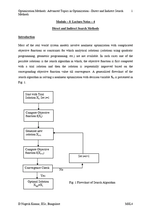
Module – 8 Lecture Notes – 4Direct and Indirect Search MethodsIntroductionMost of the real world system models involve nonlinear optimization with complicated objective functions or constraints for which analytical solutions (solutions using quadratic programming, geometric programming, etc.) are not available. In such cases one of the possible solutions is the search algorithm in which, the objective function is first computed with a trial solution and then the solution is sequentially improved based on the corresponding objective function value till convergence. A generalized flowchart of the search algorithm in solving a nonlinear optimization with decision variable X i, is presented in Fig. 1.The search algorithms can be broadly classified into two types: (1) direct search algorithm and (2) indirect search algorithm. A direct search algorithm for numerical search optimization depends on the objective function only through ranking a countable set of function values. It does not involve the partial derivatives of the function and hence it is also called nongradient or zeroth order method. Indirect search algorithm, also called the descent method, depends on the first (first-order methods) and often second derivatives (second-order methods) of the objective function. A brief overview of the direct search algorithm is presented.Direct Search AlgorithmSome of the direct search algorithms for solving nonlinear optimization, which requires objective functions, are described below:A) Random Search Method: This method generates trial solutions for the optimization model using random number generators for the decision variables. Random search method includes random jump method, random walk method and random walk method with direction exploitation. Random jump method generates huge number of data points for the decision variable assuming a uniform distribution for them and finds out the best solution by comparing the corresponding objective function values. Random walk method generates trial solution with sequential improvements which is governed by a scalar step length and a unit random vector. The random walk method with direct exploitation is an improved version of random walk method, in which, first the successful direction of generating trial solutions is found out and then maximum possible steps are taken along this successful direction.B) Grid Search Method: This methodology involves setting up of grids in the decision space and evaluating the values of the objective function at each grid point. The point which corresponds to the best value of the objective function is considered to be the optimum solution. A major drawback of this methodology is that the number of grid points increases exponentially with the number of decision variables, which makes the method computationally costlier.C) Univariate Method: This procedure involves generation of trial solutions for one decision variable at a time, keeping all the others fixed. Thus the best solution for a decision variablekeeping others constant can be obtained. After completion of the process with all the decision variables, the algorithm is repeated till convergence.D) Pattern Directions: In univariate method the search direction is along the direction of co-ordinate axis which makes the rate of convergence very slow. To overcome this drawback, the method of pattern direction is used, in which, the search is performed not along the direction of the co-ordinate axes but along the direction towards the best solution. This can be achieved with Hooke and Jeeves’ method or Powell’s method. In the Hooke and Jeeves’ method, a sequential technique is used consisting of two moves: exploratory move and the pattern move. Exploratory move is used to explore the local behavior of the objective function, and the pattern move is used to take advantage of the pattern direction. Powell’s method is a direct search method with conjugate gradient, which minimizes the quadratic function in a finite number of steps. Since a general nonlinear function can be approximated reasonably well by a quadratic function, conjugate gradient minimizes the computational time to convergence.E)Rosen Brock’s Method of Rotating Coordinates: This is a modified version of Hooke and Jeeves’ method, in which, the coordinate system is rotated in such a way that the first axis always orients to the locally estimated direction of the best solution and all the axes are made mutually orthogonal and normal to the first one.F) Simplex Method: Simplex method is a conventional direct search algorithm where the best solution lies on the vertices of a geometric figure in N-dimensional space made of a set of N+1 points. The method compares the objective function values at the N+1 vertices and moves towards the optimum point iteratively. The movement of the simplex algorithm is achieved by reflection, contraction and expansion.Indirect Search AlgorithmThe indirect search algorithms are based on the derivatives or gradients of the objective function. The gradient of a function in N-dimensional space is given by:⎥⎥⎥⎥⎥⎥⎥⎥⎥⎦⎤⎢⎢⎢⎢⎢⎢⎢⎢⎢⎣⎡∂∂∂∂∂∂=∇N x f x f x f f (21)(1)Indirect search algorithms include:A) Steepest Descent (Cauchy) Method: In this method, the search starts from an initial trial point X1, and iteratively moves along the steepest descent directions until the optimum point is found. Although, the method is straightforward, it is not applicable to the problems having multiple local optima. In such cases the solution may get stuck at local optimum points.B) Conjugate Gradient (Fletcher-Reeves) Method: The convergence technique of the steepest descent method can be greatly improved by using the concept of conjugate gradient with the use of the property of quadratic convergence.C) Newton’s Method: Newton’s method is a very popular method which is based on Taylor’s series expansion. The Taylor’s series expansion of a function f(X ) at X =X i is given by:()()()()[](i i T i i T i i X X J X X X X f X f X f −−+−∇+=21) (2) where, [J i ]=[J]|x i , is the Hessian matrix of f evaluated at the point X i . Setting the partial derivatives of Eq. (2), to zero, the minimum value of f(X ) can be obtained.()N j x X f j,...,2,1,0==∂∂ (3)From Eq. (2) and (3)[]()0=−+∇=∇i i i X X J f f(4)Eq. (4) can be solved to obtain an improved solution X i+1 []i i i i f J X X ∇−=−+11 (5)The procedure is repeated till convergence for finding out the optimal solution.D) Marquardt Method: Marquardt method is a combination method of both the steepest descent algorithm and Newton’s method, which has the advantages of both the methods, movement of function value towards optimum point and fast convergence rate. By modifying the diagonal elements of the Hessian matrix iteratively, the optimum solution is obtained in this method.E) Quasi-Newton Method: Quasi-Newton methods are well-known algorithms for finding maxima and minima of nonlinear functions. They are based on Newton's method, but they approximate the Hessian matrix, or its inverse, in order to reduce the amount of computation per iteration. The Hessian matrix is updated using the secant equation, a generalization of the secant method for multidimensional problems.It should be noted that the above mentioned algorithms can be used for solving only unconstrained optimization. For solving constrained optimization, a common procedure is the use of a penalty function to convert the constrained optimization problem into an unconstrained optimization problem. Let us assume that for a point X i , the amount of violation of a constraint is δ. In such cases the objective function is given by:()()2δλ××+=M X f X f i i (6)where, λ=1( for minimization problem) and -1 ( for maximization problem), M=dummy variable with a very high value. The penalty function automatically makes the solution inferior where there is a violation of constraint.SummaryVarious methods for direct and indirect search algorithms are discussed briefly in the present class. The models are useful when no analytical solution is available for an optimization problem. It should be noted that when there is availability of an analytical solution, the search algorithms should not be used, because analytical solution gives a global optima whereas, there is always a possibility that the numerical solution may get stuck at local optima.。

geometry optimization的定义几何优化的定义几何优化是一种数学方法，旨在寻找使得给定系统达到最佳状况的结构或形状。

该方法通常应用于科学、工程和计算机图形学领域，目的是通过调整系统的几何形状或参数，使系统具备最佳的性能。

在几何优化中，我们使用数学模型和算法来寻找给定问题的最优解。

这种方法的核心是优化算法，可以根据不同的目标和约束条件来优化几何形状。

几何形状可以是二维或三维结构，如图形、物体、建筑或分子。

几何优化被广泛应用于各种领域。

在科学研究中，它可以帮助研究人员优化实验装置的结构，以便获得更准确或更稳定的实验结果。

在工程领域，几何优化可以优化汽车、飞机或建筑物的设计，以提高其性能和效率。

在计算机图形学领域，几何优化可以用于生成逼真的图像和动画。

几何优化的基本步骤包括定义目标函数、设定约束条件、选择合适的优化算法以及优化参数的迭代过程。

目标函数通常是需要最小化或最大化的一个性能指标，如能量、距离、曲率等。

约束条件是一组限制条件，限制系统在优化过程中的变化范围。

优化算法根据定义的目标函数和约束条件，通过迭代搜索的方式寻找最优解。

几何优化的挑战在于寻找一个全局最优解或接近最优解的解。

由于问题的复杂性和多样性，很难找到一个完美的解决方案。

因此，几何优化常常需要结合经验知识和创造性思维，通过多次尝试和调整，逐步优化和改进问题的解决方案。

总结而言，几何优化是一种重要的数学方法，用于通过调整系统的几何形状或参数，寻找使系统达到最佳状态的解决方案。

它在科学、工程和计算机图形学等领域发挥着重要的作用，为问题的解决提供了有效的数学工具和计算方法。

最速下降法：算法简单，每次迭代计算量小，占用内存量小，即使从一个不好的初始点出发，往往也能收敛到局部极小点。

沿负梯度方向函数值下降很快的特点，容易使认为这一定是最理想的搜索方向，然而事实证明，梯度法的收敛速度并不快．特别是对于等值线（面）具有狭长深谷形状的函数，收敛速度更慢。

其原因是由于每次迭代后下一次搜索方向总是与前一次搜索方向相互垂直，如此继续下去就产生所谓的锯齿现象。

从直观上看，在远离极小点的地方每次迭代可能使目标函数有较大的下降，但是在接近极小点的地方，由于锯齿现象，从而导致每次迭代行进距离缩短，因而收敛速度不快.牛顿法：基本思想：利用目标函数的一个二次函数去近似一个目标函数，然后精确的求出这个二次函数的极小点，从而该极小点近似为原目标函数的一个局部极小点。

优点 1. 当目标函数是正定二次函数时，Newton 法具有二次终止性。

2. 当目标函数的梯度和Hesse 矩阵易求时，并且能对初始点给出较好估计时，建议使用牛顿法为宜。

缺点：1. Hesse 矩阵可能为奇异矩阵，处理办法有：改为梯度方向搜索。

共轭梯度法：优点：收敛速度优于最速下降法，存贮量小，计算简单.适合于优化变量数目较多的中等规模优化问题.缺点：变度量法：较好的收敛速度，不计算Hesse 矩阵1．对称秩1 修正公式的缺点（1）要求( ) ( ) ( ) ( ) ( ) 0 k k k T k y B s s − ≠0（2）不能保证B ( k ) 正定性的传递2．BFGS 算法与DFP 算法的对比对正定二次函数效果相同，对一般可微函数效果可能不同。

1） BFGS 算法的收敛性、数值计算效率优于DFP 算法；（2） BFGS 算法要解线性方程组，而DFP 算法不需要。

基本性质：有效集法：算法思想：依据凸二次规划问题的性质2，通过求解等式约束的凸二次规划问题，可能得到原凸二次规划问题的最优解。

有效集法就是通过求解一系列等式约束凸二次规划问题，获取一般凸二次规划问题解的方法。

iSIGHT优化设计—Optimization 1 概述1.1 传统劳动密集型的人工设计1.2 iSIGHT智能软件机械人驱动的设计优化1.3 优化问题特点（1）约束（3）非线性（6）组合问题（7）优化问题按特点分类对优化设计的研究不断证明，没有任何单一的优化技术能够适用于所有设计问题。

事实上，单一的优化技术乃至可能无法专门好地解决一个设计问题。

不同优化技术的组合最有可能发觉最优设计。

优化设计极大地依托于起始点的选择，设计空间本身的性质（如线形、非线形、持续、离散、变量数、约束等等）。

iSIGHT 就此问题提供两种解决方案。

第一，iSIGHT 提供完备的优化工具集，用户可交互式选用并可针对特定问题进行定制。

第二，也是更重要的，iSIGHT 提供一种多学科优化操作模式，以便把所有的优化算法有机组合起来，解决复杂的优化设计问题。

2 优化算法概述iSIGHT 包括的优化方式能够分为四大类：数值优化、全局探讨法、启发式优化法和多目标多准那么优化算法。

数值优化（如登山法）一样假设设计空间是单峰的，凸起的和持续的，本质上是一种局部优化技术。

全局探讨技术那么幸免了局限于局部区域，一样通过评估整个设计空间的设计点来寻觅全局最优。

启发式技术是按用户概念的参数特性和交叉阻碍方向寻觅最优方案。

多目标优化那么需要衡量，iSIGHT 正是提供了一种易于利用的多目标准那么衡量分析框架。

另外自iSIGHT v9.0 开始新增加了Pointer 优化器，它是GA、MPQL、N-M 单纯形法和线性单纯形法的组合。

iSIGHT 包括的具体算法按分类列表如下:2.1 数值方式iSIGHT 纳入了十二种数值优化算法。

其中八种是直接法，在数学搜索进程中直接处置约束条件。

而Exterior Penalty 方式和Hooke-Jeeves 方式是罚函数法，它们通过在目标函数中引入罚函数将约束问题转化为无约束问题。

2.2 全局探讨法iSIGHT 全局探讨法包括遗传算法和模拟退火算法，它们不受凸（凹）面性、滑腻性或设计空间持续性的限制。

optimization as a model for few-shot learning
解读
"optimization as a model for few-shot learning"是一个名词短语，其中"optimization"是主语，"as a model for few-shot learning"是作为补充说明的介词短语。

"optimization"作为一个名词，表示"the action of making the best or most effective use of a situation or resource"，在这里用作主语。

"as a model for"是一个介词短语，表示"作为...的模型"，用来说明"optimization"的作用。

"few-shot learning"是一个名词短语，表示"在少样本学习的情况下进行学习"。

总的来说，这句话使用了名词短语、介词短语和动词短语等语法结构，以表达将"optimization"作为一种模型来解决"few-shot learning"的问题。

methods 方法Methods 方法是编程中常用的一种概念，用于封装一段可重复使用的代码。

它是面向对象编程的基本组成部分之一，通过方法能够将代码逻辑进行模块化，提高代码的可维护性和重用性。

在编程中，方法是一段执行特定任务的代码块。

它可以接受输入参数，处理这些参数，并返回一个结果。

通过使用方法，我们可以将一个复杂的问题分解为多个小问题，并分别编写方法来解决这些小问题，从而简化代码的编写和维护。

在Java等面向对象的编程语言中，方法是类的成员之一。

每个类可以定义多个方法，每个方法都有一个唯一的名称和一组参数。

方法可以被其他代码调用，以完成特定的功能。

方法的定义由方法名、参数列表、返回类型和方法体组成。

方法的定义通常包含以下几个部分：1. 方法名：用于标识方法的名称，建议使用有意义的、能够描述方法功能的名称，以便于代码的阅读和理解。

2. 参数列表：用于接收传递给方法的数据，可以有零个或多个参数。

每个参数都包含一个类型和一个名称，用于指定参数的数据类型和在方法体中的使用方式。

3. 返回类型：用于指定方法的返回值类型。

方法可以有返回值，也可以没有返回值。

如果有返回值，则需要在方法定义中使用返回类型指定返回值的类型。

4. 方法体：包含了方法的具体实现逻辑。

方法体中的代码会在方法被调用时执行。

方法体可以包含各种语句和表达式，用于完成特定的功能。

方法的调用通常通过方法名和参数列表来完成。

调用方法时，需要提供与方法定义中参数列表相匹配的参数。

方法的调用可以在同一个类中进行，也可以在不同的类中进行。

使用方法具有许多优点。

首先，方法可以提高代码的可读性和可维护性。

通过将代码逻辑封装在方法中，可以使代码更加模块化，易于理解和修改。

其次，方法可以提高代码的重用性。

通过将常用的代码逻辑封装在方法中，可以在多个地方进行调用，避免重复编写相同的代码。

此外，方法还可以提高代码的可测试性。

通过将代码逻辑划分为多个方法，可以更容易地编写和执行单元测试。

正交试验优选金银花中总黄酮的最佳提取工艺湖南怀化医学高等专科学校药学系（418000） 杨志学 万 顺 张亮君提 要：目的:探索金银花中总黄酮最佳提取工艺。

方法:采用正交法考察乙醇浸泡浓度，萃取时间、乙醇洗脱浓度，物料比4个因素对金银花中总黄酮得率的影响。

结果:金银花中总黄酮的最佳提取工艺；用30倍于样品重的80%的乙醇浸泡24h后继用超声法提取40min，以60%的乙醇洗脱。

结论 以超声波法提取的总黄酮含量高，操作简便，节省燃料和时间，提取较完全，此法宜工业化生产。

关键词：金银花；总黄酮；超声波；提取工艺；正交试验中图分类号：R284.2 文献标识码：B 文章编号：1006－6810（2004）05－0186－03Study on Extracition process of flavonoids In Flos by the method of orthogonal test optimization.Yang Zhi-xue Wan Shun.Zhang Liang-jun lpharmaceutical Department,Huaihua Medical College Huaihua 418000)Abstract:OBJE CTIVE:study on extro ction process of flovonoids in Flos Lonicerae. METHODS:The orthogonal test was adopted to ve search the effects of 4 factors on the yielding rate of flavo noids from flos lonicerae, RESULTS:The concentration of 80% ethanol was 30 times raw herbtodouse the dried the dried flos Lonicevae for 24 hours,and altrasonic treatment lasted for ane hour.The extraction of flavonoids was as high as 3.2%.CONLUSION:This process is characterized with simple operation safe operate save of fuel and time.So this technology is guitable for in dustrialized prodaction.KEY WORD:Flos Lonicerae;gross flavonoids; process altrasonic Extraction process; orthogonal test.金银花为忍冬科植物忍冬 Lonicera japonica Thumb.的干燥花蕾，为临床常用中药，具有清热解毒，凉散风热之攻效，主治痈肿疗疮、喉痹、丹毒、热毒血痢、风热感冒、温病发势等[1]。